Why (Graph) DBMSs Need New Join Algorithms

The Story of Worst-case Optimal Join Algorithms

Joins on a set of records is objectively the most expensive operation in DBMSs. In my previous post on , I said that in the field of databases, once in a while you run into a very simple idea that deviates from the norm that gets you very excited. Today, I will discuss another such idea, worst-case optimal join (wcoj) algorithms. Wcoj algorithms and the theory around it in one sentence says this:

Queries involving complex “cyclic joins” over many-to-many relationships should be evaluated column at a time instead of table at a time, which is the norm.

Wcoj algorithms find their best applications when finding cyclic patterns on graphs, such as cliques or cycles, which is common in the workloads of fraud detection and recommendation applications. As such, they should be integrated into every graph DBMS (and possibly to RDBMSs) and I am convinced that they eventually will.

TL;DR: The key takeaways are:

History of Wcoj Algorithms: Research on wcoj algorithms started with a solution to open question about the maximum sizes of join queries. This result made researchers realize this: the traditional “binary join plans” paradigm of generating query plans that join 2 tables a time until all of the tables in the query are joined is provably suboptimal for some queries. Specifically, when join queries are cyclic, which in graph terms means when the searched graph pattern has cycles in it, and the relationships between records are many-to-many, then this paradigm can generate unnecessarily large amounts of intermediate results.
Core Algorithmic Step of Wcoj Algorithms: Wcoj algorithms fix this sub-optimality by performing the joins one column at a time (instead of 2 tables at a time) using multiway intersections.
How Kùzu Integrates Wcoj Algorithms: Kùzu generates plans that seamlessly mix binary joins and wcoj-style multiway intersections. Multiway intersections are performed by an operator called “multiway HashJoin”, which has one or more build phases that creates one or more hash tables that stores sorted adjacency lists; and a probe phase that performs multi-way intersections using the sorted lists.
Yes, the Term “Worst-case Optimal” Is Confusing Even to Don Knuth: I know, Don Knuth also found the term “worst-case optimal” a bit confusing. See my anecdote on this. It basically means that the worst-case runtimes of these algorithms are asymptotically optimal.

Joins, Running Example & Traditional Table-at-a-time Joins

Joins are objectively the most expensive and powerful operation in DBMSs. In SQL, you indicate them in the FROM clause by listing a set of table names, in Cypher in the MATCH clause, where you draw a graph pattern to describe how to join node records with each other. As a running example, consider a simple social network of users and followers, whose node-link diagram is shown below. I am also showing the table that contains these records in a User (ignore the name property for now) and Follows tables.

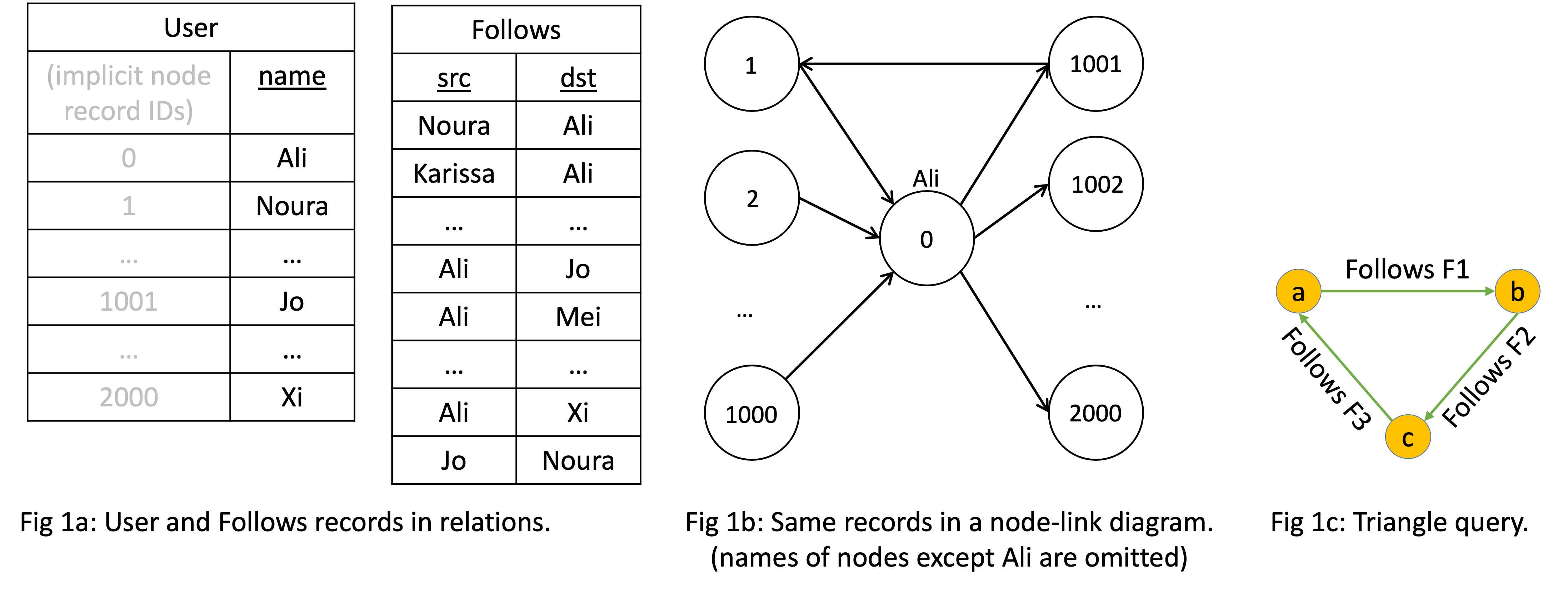
Consider finding triangles, which is one of the simplest forms of cycles and cliques, in this network. The SQL and Cypher versions of this query are shown below.

SQL

SELECT *
FROM  Follows f1, Follows f2, Follows f3
WHERE f1.dst=f2.src AND f2.dst=f3.src AND
      f3.dst = f1.src

Cypher

MATCH (a:User)-[f1:Follows]->(b:User)-[f2:Follows]->(c:User)-[f3:Follows]->(a)
RETURN *

That long MATCH clause “draws” a triangle and for our case here, this is equivalent to joining three copies of the Follows table.

Now ever since the System R days and Patricia Selinger’s 1979 seminal paper that described how System R compiled and optimized SQL queries, there has been an unchallenged dogma in DBMSs that the joins specified in the query would be evaluated pairwise, table at a time. Here’s a blurb from Selinger’s paper, where one can see this assumption: ”In System R a user need not know how the tuples are physically stored … Nor does a user specify in what order joins are to be performed. The System R optimizer chooses both join order and …” To this day, this is the norm. DBMSs pick a “join order” which is the order in which the tables should be joined iteratively 2 at a time. In the above example, for example there are three possible join orders. One way to represent these orders is by writing different parenthesization of the joins:

(i) $((F1 \bowtie F2) \bowtie F3)$ ;
(ii) $(F1 \bowtie (F2 \bowtie F3))$ ;
(iii) $((F1 \bowtie F3) \bowtie F2)$ .

The optimization problem for a system is of course more complex than just ordering tables because the system also has to choose which binary join algorithm to use when joining each pair of tables, e.g., hash joins vs merge joins. But take any system you want, and they will all follow the same paradigm of joining 2 base or intermediate tables iteratively, until all tables are joined: hence the term binary joins to describe the plans of existing systems.

A Math Puzzle That Started it All

So, what’s the problem with binary join plans? When join queries are cyclic and the relationships are many-to-many, they can generate provably large amounts of (so unnecessary in a formal sense) intermediate results. First, cyclicity for join queries has formal (and a bit intimidating) definitions but if you think of graph patterns, it simply means that the searched pattern’s undirected version has cycles. Why do binary joins generate unnecessarily large intermediate results? I’ll get to this below but first a bit of history on the origins of this insight. The whole topic of “worst-case optimal joins” started with 2 papers, a 2007 SODA and a 2008 FOCS paper, which are top venues in algorithms and theory. In these papers, several theoreticians solved a fundamental open question about join queries. Suppose I give you:

An arbitrary natural join query, say of $m$ relations. In DBMS literature we denote such queries as $Q=R1(a_{11}, ..., a_{r1}) \bowtie ... \bowtie Rm(a_{m1}, ..., a_{rm})$ .
Sizes of R1, …, Rm, e.g., for simplicity assume they all have $IN$ many tuples.

“Natural” here means that the join predicates are equality predicates on identical column names. You, as the second person in this puzzle, are allowed to set the values inside these relations. The open question was: how large can you make the final output? So for example, if I told you that there are $IN$ many tuples in the Follows tables, what is the maximum number of triangle outputs there can be?¹ Even more concretely for the triangle query, the question is: out of all possible graphs with $IN$ many edges, what is the maximum number of triangles they contain?

It still surprises me that the answer to this question was not known until 2008. It just looks like a fundamental question someone in databases must have answered before. Now excuse me for bombarding your brains with some necessary math definitions. These two papers showed that the answer is: $IN^{\rho^*}$ , where $\rho^*$ is a property of $Q$ called the fractional edge cover number of $Q$ . This is the solution to an optimization problem and best explained by thinking about the “join query graph”, which, for our purposes, is the triangle graph pattern (ignoring the edge directions), shown in Fig 2a and 2b.

The optimization problem is this: put a weight between [0, 1] to each “query edge” such that each “query node” is “covered”, i.e., the sum of the query edges touching each query node is > 1. Each such solution is called an edge cover. The problem is to find the edge cover whose total weight is the minimum. That is called the fractional edge cover number of the query. For the triangle query, one edge cover, shown in Fig 2a, is [1, 1, 0], which has a total weight of 1 + 1 + 0 = 2. The minimum weight edge cover is [1/2, 1/2, 1/2], shown in Fig 2b, with a total weight of 1.5. Therefore, the fractional edge cover number $\rho^*$ of the triangle query is 1.5. In general, each edge cover is an upper bound but the FOCS paper showed that the fractional edge cover number is the tight upper bound. So the maximum number of triangles there can be on a graph with $IN$ edges is $\Theta(IN^{1.5})$ and this is tight, i.e., there are such graphs. Nice scientific progress! Nowadays, the quantity $IN^{\rho^*}$ is known as the AGM bound of a query, after the first letters of the last names of the authors of the FOCS paper.

Problem With Table-at-a-time/Binary Joins

Now this immediately made the same researchers realize that binary join plans are provably sub-optimal because they can generate polynomially more intermediate results than the AGM bound of the query. This happens because on cyclic queries, the strategy of joining tables 2 at a time may lead to unnecessarily computing some acyclic sub-joins. For example, in the triangle query, the plan $((F1 \bowtie F2) \bowtie F3)$ first computes $(F1 \bowtie F2)$ sub-join, which in graph terms computes the 2-paths in the graph. This is a problem because often there can be many more of these acyclic sub-joins than there can be outputs for the cyclic join. For this plan, there can be $IN^2$ many 2-paths (which is the AGM bound of 2-paths), which is polynomially larger than $IN^{1.5}$ . For example in our running example, there are 1000*1000 = 1M many 2 paths, but on a graph with 2001 edges there can be at most 89.5K triangles (well ours has only 3 triangles (because the triangle query we are using is symmetric the sole triangle would generate 3 outputs for 3 rotations of it)).

Any other plan in this case would have generated $IN^2$ many 2-paths, so there is no good binary join plan here. I want to emphasize that this sub-optimality does not occur when the queries are acyclic or when the dataset does not have many-to-many relationships. If the joins were primary-foreign key non-growing joins, then binary join plans will work just fine.

Solution: Column-at-a-time “Worst-case Optimal” Join Algorithms

So the immediate next question is: are there algorithms whose runtimes can be bounded by $O(IN^{1.5})$ ? If so, how are they different? The answer to this question is a bit anti-climactic. The core idea existed in the 2007 SODA and 2008 FOCS papers, though it was refined more ~4 years later in some theoretical papers by Hung Ngo, Ely Porat, Chris Ré, and Atri Rudra in the database fields PODS and SIGMOD Record. The answer is simply to perform the join column at a time, using multiway intersections. “Intersections of what?” you should be asking. For joins over arbtrary relations, we need special indices but I want to skip this detail. In the context of GDBMSs, GDBMSs already have join indices (aka adjacency list indices) and for the common joins they perform, this will be enough for our purposes.

I will next demonstrate a wcoj algorithm known as “Generic Join” from the SIGMOD Record paper. It can be seen as the simplest of all wcoj algorithms. As “join order”, we will pick a “column order” instead of Selinger-style table order. So in our triangle query, the order could be a,b,c. Then we will build indices over each relation that is consistent with this order. In our case there are conceptually three (identical) relations: Follows1(a, b), Follows2(b, c), Follows3(c, a). For Follows1, we need to be able to read all b values for a given a value (e.g., a=5). In graph terms, this just means that we need “forward join index”. For Follows3, because a comes earlier than c, we will want an index that gives us c values for a given a value. This is equivalent to a “backward join index”. In graphs, because joins happen through the relationship records, which can, for the purpose of the joins, be taught of as a binary relation (src, dst), 2 indices is enough for our purposes. On general relations, one may need many more indices.

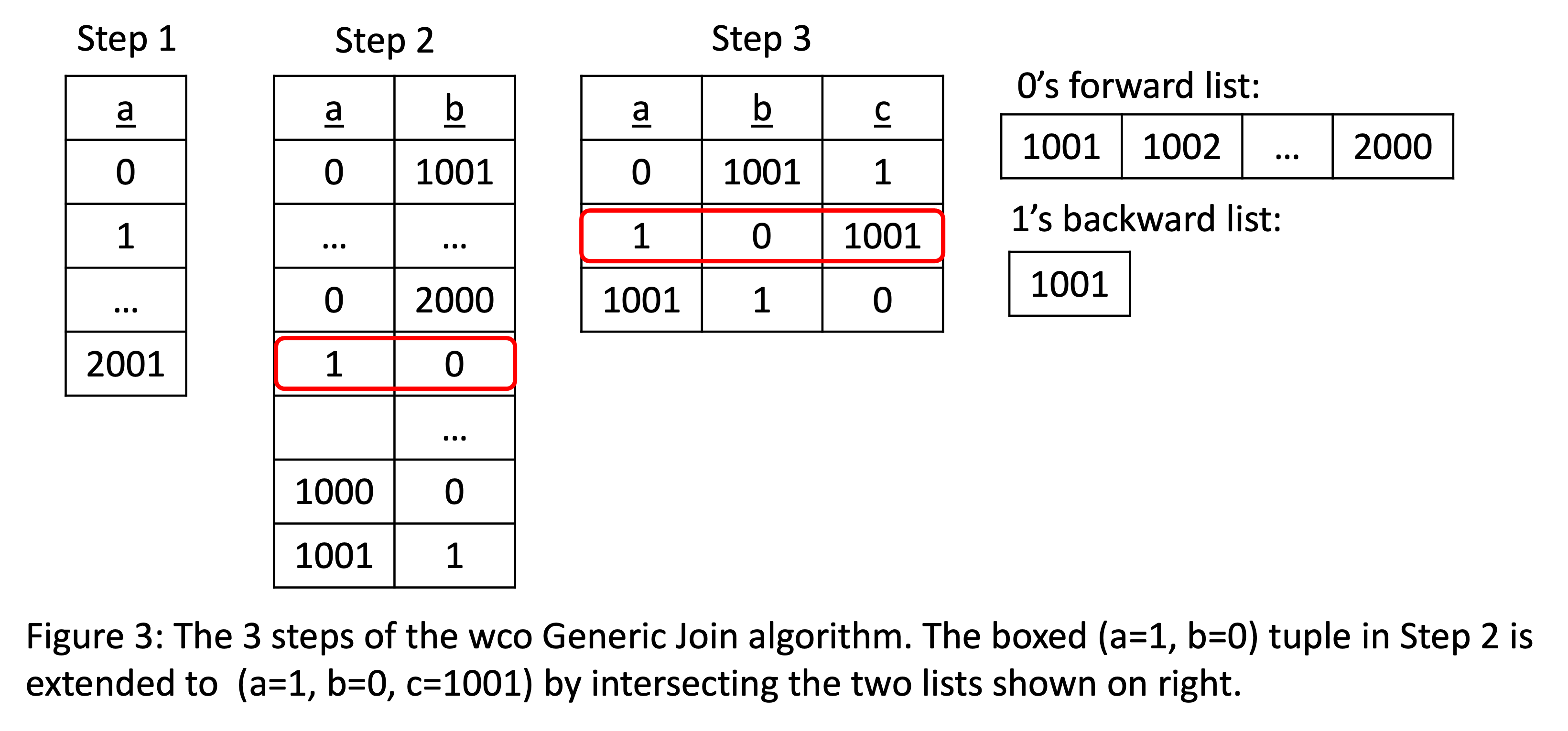
We will iteratively find: (i) all a values that can be in the final triangles; (ii) all ab’s that be in the final triangles; and (iii) all abc’s, which are the triangles. Let’s simulate the computation:

Step 1: Find all a‘s. Here we will just take all nodes as possible a values. This is shown under “Step 1” in the above figure.
Step 2: For each a value, e.g., a=1, we extend it to find all ab’s that can be part of triangles: Here we use the forward index to look up all b values for node with ID 1. So on and so forth. This will generate the second intermediate relation.
Step 3: For each ab value, e.g., the tuple (a=1 b=0), we will intersect all c’s with a=1, and all c’s with b=0. That is, we will intersect the backward adjacency list of the node with ID 1, and forward adjacency list of the node with ID 0. If the intersection is non-empty, we produce some triangles. In this case, we will produce the triangle (a=1, b=0, c=1001) The result of this computation will produce the third and final output table in the figure.

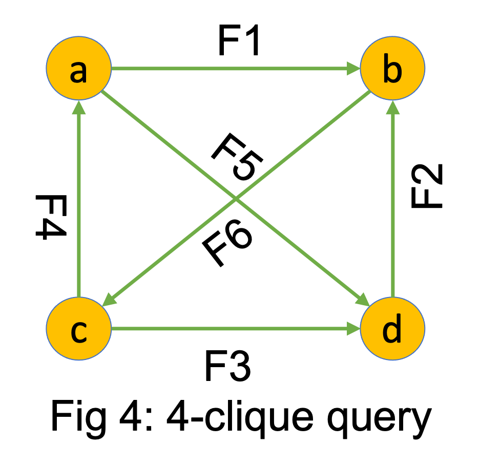
Note that this process did not produce the 2-paths as an intermediate step, which is how wcoj algorithms fix for the sub-optimality of binary join algorithms. If your query was more complex then a wcoj algorithm can do k-way intersections where k > 2. For example on the 4-clique query shown on the right, suppose the column order is abcd, then given abc triangles, we would do a 3-way intersection of forward index of a’s, backward index of b’s, and forward index of c’s, to complete the triangles to joins. This type of multiway intersections is the necessary algorithmic step to be efficient on cyclic queries.

How Kùzu Performs Worst-case Optimal Join Algorithms:

Our CIDR paper describes this in detail, so I will be brief here. First, Kùzu mixes binary joins and wcoj-like multiway intersections following some principles that my PhD student Amine Mhedhbi had worked quite hard on early in his PhD. I recommend these two papers, one by Amine and me and one by the Umbra group on several different ways people have proposed for mixing binary and wcoj algorithms in query plans. Overall message of these studies is that, wcoj are critical when the query has a very cyclic component and multiway intersections can help. If the query does not have this property, systems should just use binary joins. So wcoj-like computations should be seen as complementing binary join plans.

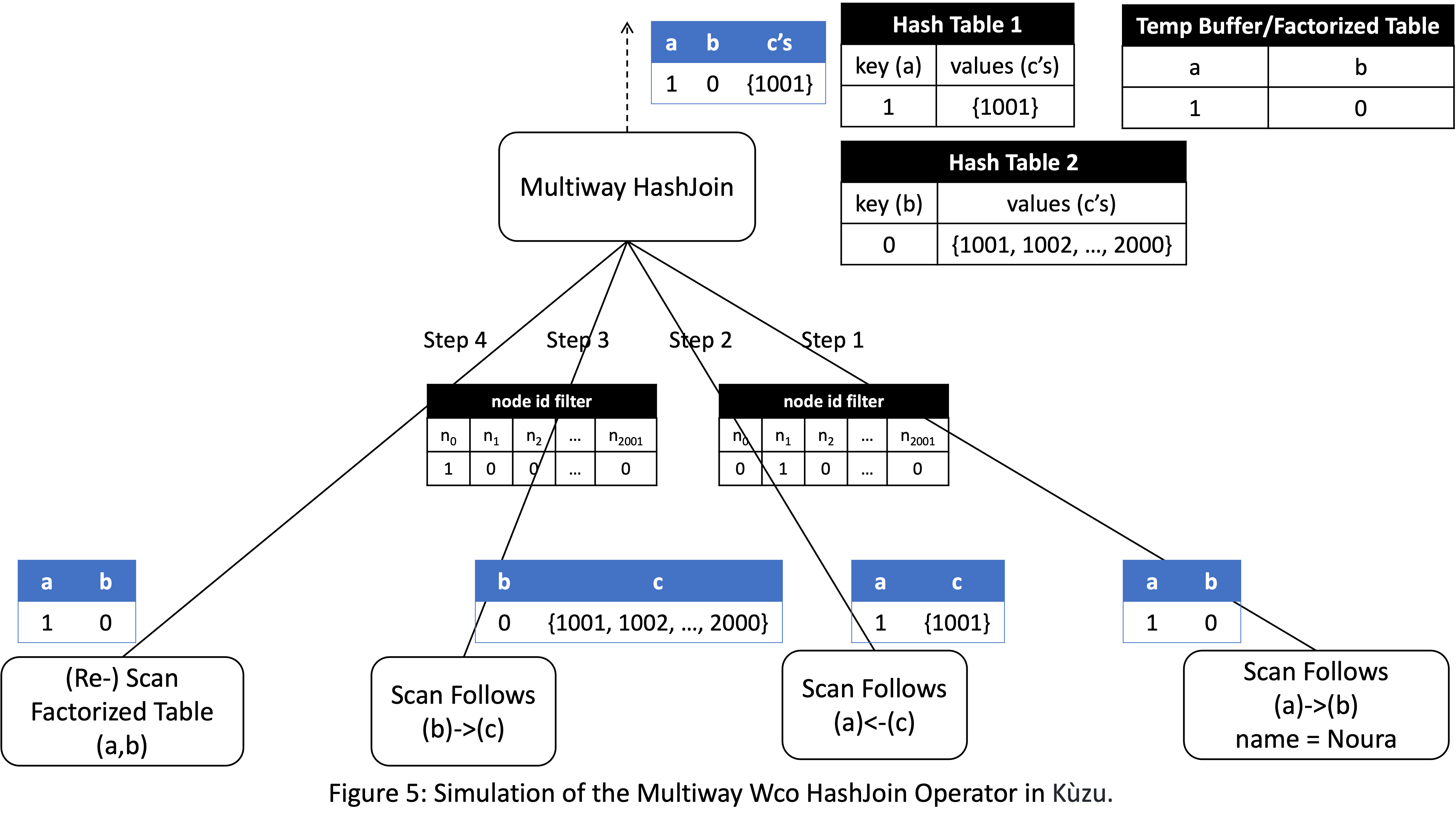
Second, Kùzu performs multiway intersections in a Multiway HashJoin operator. In our CIDR paper we call this operator Multiway ASPJoin. It can be thought of a modified hash-join operator where we use multiple hash tables and do an intersection to produce outputs as I will simulate. Let me change the query a little and add a filter on a.name = Noura, where name is the primary key of User records. You can see from Fig 1a that Noura is the primary key of node with ID 1. In my simulation, the Multiway HashJoin operator will take ab tuples and extend them to abc tuples through a 2-way intersection. In general multiway HashJoin has 3 phases: 1 accumulate phase, build phases to build k-2 hash tables, and a probe phase. Here are the steps.

Accumulate Phase: The operator receives the ab tuples which will be extended to triangles. This allows the system to see exactly the forward/backward lists of which nodes will be intersected. Then, the operator passes this information sideways to only scan those lists. In this case, because there is a primary key filter on Noura, the only ab tuple that will be read is (a=1,b=0). This is stored in a temporary buffer that we call “Factorized Table” in the system.
Build Phase 1: In the first build step, Multway HashJoin will pass a nodeID filter to the Scan Follows (a)<-(c) operator with only 1=true for node ID 1, and 0 for every other node ID. The operator can do this because at this stage the operator knows exactly which backward adjacency lists will be needed when we extend the tuple (in this case only node with ID 1’s backward list is needed). The Scan operator uses this node ID filter to scan only this backward list, {1001}, and avoids scanning the rest of the file that stores the backwards Follows edges. This list is first sorted based on the IDs of the neighbor IDs and stored in a hash table, denoted as “Hash Table (a)<-(c)” in the figure.
Build Phase 2: This is similar to Build phase 1. Using a semijoin filter with node 0’s ID, we scan only node 2’s forward Follows list {1001, 1002, …, 2000}, sort it, and then store in a hash table “Hash Table (b)->(c)“.
Probe: We re-scan the accumulated ab tuples from the factorized table. For each tuple, we first probe “Hash Table (a)<-(c)” and then “Hash Table (b)->(c)” to fetch two lists, intersect them, and produce outputs. In this case there is only one tuple (a=1, b=0), so we will fetch a=1’s backward list and b=0’s forward list, intersect these lists, and produce the triangle (a=1, b=0, c=1001).

This performs quite well. Our CIDR paper has some performance numbers comparing against other types of WCO joins implementations (see the experiments in Table 3). Since I did not cover other ways to implement wco join algorithms inside DBMSs, these experiments would be difficult to explain here. Instead, let me just demonstrate some simple comparisons between using binary joins and wco joins in Kùzu on a simple triangle query. On larger cyclic queries, e.g., 4- or 5- cliques, the differences are much larger and often binary join plans do not finish on time. You can try this experiment too.

Here is the configuration. The dataset I’m using is a popular web graph that is used in academic papers called web-BerkStan. It has 685K nodes and 7.6M edges. I modeled these as a simple Page nodes and Links edges.

I start Kùzu on my own laptop, which is a Macbook Air 2020 with Apple M1 chip, 16G memory, and 512GB SSD, and run the following two queries (by default, Kùzu uses all available threads, which is 8 in this case):

// Q1: Kùzu-WCO
MATCH (a:Page)-[e1:Links]->(b:Page)-[e2:Links]->(c:Page)-[e3:Links]->(a)
RETURN count(*)

This will compile plan that uses a wco Multiway HashJoin operator. I will refer to this plan as Kùzu-WCO below. I am also running the following query:

// Q2: Kùzu-BJ
MATCH (a:Page)-[e1:Links]->(b:Page)
WITH *
MATCH (b:Page)-[e2:Links]->(c:Page)
WIH *
MATCH (c)-[e3:Links]->(a)
RETURN count(*)

Currently Kùzu compiles each MATCH/WITH block separately so this is hack to force the system to use binary join plan. The plan will join e1 Links with e2 Links and then join the result of that with e3 Links, all using binary HashJoin operator. I will refer to this as Kùzu-BJ. Here are the results:

Configuration	Time
Kùzu-WCO	1.62s
Kùzu-BJ	51.17s

There are ~41M triangles in the output. We see 31.6x performance improvement in this simple query. In larger densely cyclic queries, binary join plans just don’t work.

To try this locally, you can download our prepared CSV files from here, and compile from our latest master² — use the command make clean && make release NUM_THREADS=8. Then start a Kùzu shell, and load data into Kùzu:

./build/release/tools/shell/kuzu_shell -i web.db
kuzu> CREATE NODE TABLE Page (id INT64, PRIMARY KEY(INT64));
kuzu> CREATE REL TABLE Links (FROM Page TO Page, MANY_MANY);
kuzu> COPY Page FROM 'web-node.csv';
kuzu> COPY Links FROM 'web-edge.csv';

Now, run those two queries (Kùzu-WCO and Kùzu-BJ) to see the difference!

A thank you & an anecdote about Knuth’s reaction to the term “Worst-case Optimal”

Before wrapping up, I want to say thank you to Chris Ré, who is a co-inventor of earliest wcoj algorithms. In the 5th year of my PhD, Chris had introduced me to this area and we had written a paper together on the topic in the context of evaluating joins in distributed systems, such as MapReduce and Spark. I ended up working on these algorithms and trying to make them performant in actual systems for many more years than I initially predicted. I also want to say thank you to Hung Ngo and Atri Rudra, with whom I have had several conversations during those years on these algorithms.

Finally, let me end with a fun story about the term “worst-case optimal”: Several years ago Don Knuth was visiting UWaterloo to give a Distinguished Lecture Seminar, which is our department’s most prestigious lecture series. A colleague of mine and I had a 1-1 meeting with him. Knuth must be known to anyone with a CS degree but importantly he is credited for founding the field of algorithm analysis (e.g., for popularizing the big-oh notation for analyzing algorithms’ performances). In our meeting, he asked me what I was working on and I told him about these new algorithms called “worst-case optimal join algorithms”. The term was so confusing to him and his immediate interpretation was: “Are they so good that they are optimal even in their worst-case performances?”

The term actually means that the worst-case runtime of these algorithms meets a known lower bound for the worst-case runtime of any join algorithm, which is $\Omega(IN^{\rho^*})$ . Probably a more standard term would be to call them “asymptotically optimal”, just like people call sort merge an asymptotically optimal sorting algorithm under the comparison model.

Final words

What other fundamental algorithmic developments have been made in the field on join processing? It is surprising but there are still main gaps in the field’s understanding of how fast joins can be processed. There has been some very interesting work in an area called beyond worst-case optimal join algorithms. These papers ask very fundamental questions about joins, such as how can we prove that a join algorithm is correct, i.e., it produces the correct output given its input? The high-level answer is that each join algorithm must be producing a proof that its output is correct, through the comparison operations it makes. The goal of this line of research is to design practical algorithms whose implicit proofs are optimal, i.e., as small as possible. This is probably the most ambitious level of optimality one can go for in algorithm design. There are already some algorithms, e.g., an algorithm called Tetris. The area is fascinating and has deep connections to computational geometry. I advised a Master’s thesis on the topic once and learned quite a bit about computational geometry that I never thought could be relevant to my work. The current beyond worst-case optimal join algorithms however are currently not practical. Some brave souls need to get into the space and think hard about whether practical versions of these algorithms can be developed. That would be very exciting.

This completes my 3-part blog on the contents of our CIDR paper and 2 core techniques: factorization and worst-case optimal join algorithms that we have integrated into Kùzu to optimize for many-to-many joins. My goal in these blog posts was to explain these ideas to a general CS/software engineering audience and I hope these posts have made this material more approachable. My other goal was to show the role of theory in advancing systems. Both of these ideas emerged from pen-and-paper theory papers that theoreticians wrote but gave clear advice to DBMS developers. As I said many times, I’m convinced that among many other techniques, these two techniques need to be integral to any GDBMS that wants to be competitive in performance, because queries with many-to-many joins are first-class-citizens in the workloads of these systems.

We will keep writing more blog posts in the later months about our new releases, and other technical topics. If there are things you’d like us to write about, please reach out to us on Discord! Also please give Kùzu a try, prototype applications with it, break it, let us know of your performance or other bugs, so we can continue improving it. Also give us a star on GitHub, and take care until the next post!

The question is interesting in the set semantics when you cannot pick every column value of every tuple the same value, which forces a Cartesian product of all the relations. ↩
We found a minor bug in the latest release 0.0.2 when a node has a very large number of edges, which is fixed in the master branch, that’s why we suggest using the master branch. ↩