Vector Indices Explained Through the FES Theorem

Vectors, which are high-dimensional embeddings of objects, such as text documents or images, are used in a wide range of modern LLM-based/agentic applications. Vector indices (1, 2, 3), which quickly find a set of vectors that are similar to each other are becoming a core part of many modern data systems. Since version 0.9.0, Kuzu also ships with its own native vector index. Our design allows users to do arbitrary hybrid graph and vector search, a capability many applications need to bring context and precision to their vector retrievals. Soon, my amazing student Gaurav and I will write about Kuzu’s vector index design, which is based on an upcoming VLDB 2025 paper. Today, as a precursor to that post, I will write about the foundations of a particular vector index design called hierarchical navigable small worlds (HNSW) indices (1, 2). This is the design used by most modern vector indices in practice and also the one Kuzu uses.

This post is based on several lectures from a graduate course that I gave last fall at University of Waterloo. My goal is to explain HNSW indices as an evolution of two other earlier vector indices, kd trees and sa trees. These all fall under graph/tree-based indices, where the index itself is a graph of nodes/vectors that are connected to other vectors. There are three core ideas behind HNSW indices:

Connecting pairs of close vectors with each other in the index;
Neighborhood pruning optimization; and
KNN search algorithm;

As I will explain, these ideas exist in kd trees and sa trees. My goal is that by explaining HNSW in light of kd trees and sa trees, the HNSW design will look more intuitive to people.

To help position the capabilities of these three indices, I will also use a framework that I refer to as the “FES theorem”¹, which is the observation that any vector index can provide at most two of the following three properties:

Fast, i.e., given a query vector $q$ , returns vectors that are similar to $q$ quickly, e.g., in ms latency;
Exact results, i.e., given $q$ , correctly returns the most similar vectors to $q$ (instead of “approximate” indices that can make some mistakes); and
Scalable, i.e., the index can store and search high-dimensional vectors, say 100s or 1000s of dimensions instead or 2D or 3D vectors.

The indices I cover capture each possible 2 combinations of these three properties as summarized below:

Index	F	E	S
kd trees	✅	✅	❌
sa trees	❌	✅	✅
HNSW	✅	❌	✅✅

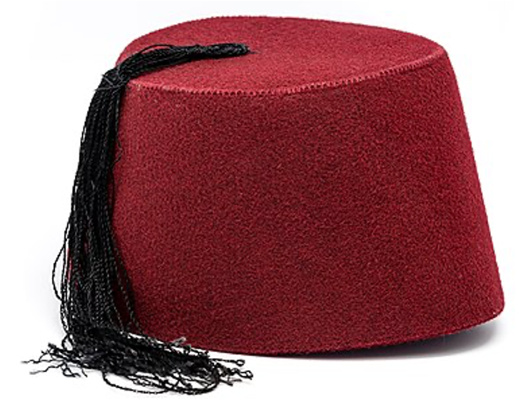
You’ll notice that my choice of the term “FES theorem” intentionally echoes the the famous CAP theorem of distributed systems that “states that any distributed data store can provide at most two of the following three guarantees: Consistency, Availability, and Partition tolerance.” Some of you will also notice that just like cap, fes (Turkish) or fez (English) is a type of headdress. Now you see why I had to pick the term.²

High-level Problem: Vector Search

The high-level search problem vector/spatial indices solve is the following. We are given as input:

(i) a set of vectors $V$ , which are points in some space that could be 2D, 3D, or a 1000 dimensional one³; and

(ii) a query vector $q$ in the same space.

The goal is to find vectors in $V$ that are close to $q$ . There are several variants of the problem, such as finding the $k$ -nearest neighbors (kNN query) of $q$ or finding all points that is within a radius $r$ of $q$ (range query). The problem is quite hard, especially when the input vectors have high dimensions because of a geometric phenomenon known as the curse of dimensionality, which is that in high-dimensional spaces pairs of vectors seem to have similar distances⁴. To make the matters worse, computing distances, say the L2 or cosine distance, of two high-dimensional vectors is expensive. This generally requires expensive vector multiplications. So the goal is that given $q$ , the index should compute distances to as few vectors in $V$ as possible to answer the kNN or range query.

I’ll focus on kNN queries in this post but exactly the same ideas are used to answer range queries. As in any index, such as a B+ tree index, the goal of a vector index is to organize the vectors in some data structure so that answering queries is fast.

Kd Tree

Kd trees are balanced trees that organize vectors by recursively dividing the space into two equal-sized partitions along one of the dimensions. Let’s suppose we have the following 2D vectors on the left.

We first split along one dimension, say the x dimension. That is, we sort the vectors according to their x-axis values and then find the median vector. In our example, the median x value is 5 (the thick red line), so the point (5,3) is picked. We put all points with x-value $\le 5$ to the left partition, and all vectors with x-value $> 5$ to the right. Then we recursively take the left and right partitions one at a time and split each one into two further equal partitions so that the tree remains balanced. Although not strictly necessary, the common wisdom is to switch the dimensions in a round robin fashion when picking the next set of median vectors. However, the main goal is to recursively split the vectors equally along some dimension. In our example, we would then split the left partition using the (2, 2) vector (so along the y=2 line) and the right partition using the (9, 5) vector (so along the y=5 line), so on and so forth. The final kd tree that we construct is shown on the right above.

Let’s next look at the kNN search algorithm. This is a simple brute-force algorithm with a simple heuristic. We are given a query vector $\texttt{q}$ and a value $\texttt{k}$ . I’m assuming that there is a function $\texttt{dist}$ that we can use to compute the distance between two vectors. Let $\texttt{T}$ be the kd tree. Below is the pseudocode of the algorithm. In the rest of the post, I’ll be using the term “to explore a vector v” to mean to compute its distance to q.

kNNSearch(q, k):
     // results stores (v, d) pairs, where v is an "explored" vector whose distance to q is d.
01.  results = max priority queue 
     // candidates stores (c, lb) pairs, where c is a candidate vector and lb is a lower bound 
     // on the distance of q to every node in the subtree rooted at c (including c). 
02.  candidates = min priority queue
03.  entry = T.root
04.  candidates.put(entry, lb=0)
05.  while (!candidates.empty()):
        // get the next candidate vector, i.e., the one whose subtree of vectors 
        // has the smallest lower bound to q
06.    (c, lb) = candidates.popMin()
07.    if (results.size() < k or lb < results.peekMax().d):
         // explore the candidate c
08.      dist_q_c = dist(q, c)
09.      if (results.size() < k):
10.        results.put((c, dist_q_c))
11.      else if (dist_q_c < results.peekMax().d):
12.        results.popMax()
13.        results.put((c, dist_q_c))
14.      for (child in c.children):
           // assume splitting dimension of candidate c is x; similar computation
           // would be done if the splitting dimension is another dimension.
16.        child_lb = 0
17.        if (child is the left child): 
18.          child_lb = c.x < q.x ? q.x - c.x : 0
19.        else:
20.          child_lb = c.x > q.x ? c.x - q.x : 0
21.        candidates.put(child, child_lb)

I am calling this a brute-force algorithm because I can summarize it as follows: starting from the root,
search the entire kd tree similar to any graph search algorithm like BFS, DFS, or A*. During the search keep track of 2 things:

candidates priority queue: Just like in any graph search algorithm, keep track of the set of nodes in the “frontier” of the graph search. These are the nodes whose neighbors will be visited next.
results priority queue: The k nearest neighbors we have explored so far, i.e., whose distances have already been computed.

That’s really the core of the algorithm. The full algorithm improves this brute-force algorithm with one optimization and one heuristic:

Subtree skipping optimization: If a subtree rooted at node $\texttt{c}$ cannot contain any vectors that can be in the k nearest neighbor of $\texttt{q}$ , then the algorithm just skips exploring this entire subtree.
Lowest-lower-bound-first heuristic: At each step, the algorithm picks to explore the candidate vector whose subtree has the smallest lower bound to $q$ . This optimization captures the intuition that subtrees with high lower bound values are likely to contain vectors that are far from q, so less likely to contain the k nearest neighbors of $q$ . This is implemented in the (c, lb) = candidates.popMin() code on line 6.

Perhaps the more interesting question is: how can we compute the lower bound of $q$ to all the nodes in the subtree rooted at a node $c$ ? This is also quite intuitive. Take for example the query (3, 6) shown as a green dot in the figure above. Consider further the subtree rooted at (9, 5) in the kd tree. This subtree was created when we were splitting the vectors along the $x=5$ line using the (5, 3) median point. Further, this subtree contained all the vectors with x-value $> 5$ . Since every vector in this space has an x-value $> 5$ , assuming our $\texttt{dist}$ function is the Euclidean distance, the minimum distance of $q$ to any vector in this subtree is 5-3=2 (since the x value of $q$ is 3)⁵. That’s all.

By construction of the kd tree and the brute-force nature of the search algorithm, kd trees are exact. Further, on small-dimensional vectors, 2D or 3D, they are also fast because the lower bounds they put can be quite effective. This is because, each dimension has a significant contribution to the overall distances between vectors. So even a lower bound obtained by using the distance along a single dimension can be effective. Therefore, the “subtree skipping optimization” works well and ends up skipping many subtrees. Since the tree is balanced and each node has only 2 children, subtrees can contain very large numbers of vectors, especially at the higher levels of the tree. Therefore, skipping subtrees can skip very large numbers of vectors.

For these reasons, kd trees are a great solution for searching geo-spatial data, such as longitudes and latitudes of places, which are represented by small-dimensional vectors. But as soon as your vectors have say 10 dimensions or more, the curse-of-dimensionality kicks in and the lower bounds become less effective. Therefore, in the framework of the FES theorem, kd trees are “Fast” and “Exact”, but not “Scalable”.

S-a Tree

The next index I’ll cover is the sa tree. Even though sa trees are not used in practice, it is important to cover them for two reasons. First, the sa tree contains the core idea behind “neighborhood pruning” optimization that is used in HNSW indices. Second, if you’re in research, the sa tree paper is an excellent read! This is the kind of paper that makes me say “I wish I wrote this one”.

Sa trees try to address two limitations of kd trees. First is that kd trees work only for the Euclidean distance metric. In contrast, sa trees work with arbitrary distance functions, such as L2 or cosine or even arbitrary metric spaces. Second, sa trees are designed to support vectors with higher number of dimensions. When the dimensions of a space is high, dividing it into two partitions along a median vector in one dimension will not be very effective in putting meaningful lower-bounds on the subtrees. This is because when there are hundreds of dimensions, the total contribution of any dimension to the final distance between two vectors is minimal. Therefore, the lower bounds computed to the subtrees become too loose and the subtree skipping optimization does not work. As a result, the brute-force kNN search algorithm from above really becomes brute force, i.e., explores all or close to all vectors in the index.

To address this problem, the sa tree partitions the vectors recursively into many clusters (not just 2), as follows:

S-a Tree Construction Algorithm:

Start with an arbitrary vector $r$ as the root of the tree.
Find a maximal set of vectors $C=\{c_1,...,c_t\}$ with the following neighbor diversity property: Each $c_i$ is closer to $r$ than to any other $c_j$ .
Partition the remaining vectors into $P_1$ , …, $P_t$ , such that each vector $v_i \in P_i$ is closer to $c_i$ than to any other $c_j$ . Note that $v_i$ must also be closer to $c_i$ than $r$ . This is because, otherwise, it would have been in the set $C$ .
Recursively, use steps 1-3 to construct the subtree rooted at $c_i$ using the vectors in $P_i$ .

Similar to kd trees, as you go down in an sa tree, each subtree contains vectors that are closer and closer to each other. At each step, instead of using a median vector, which partitions vectors into two parts, sa trees use a cluster of centroids $c_1, ..., c_t$ to form $t$ many partitions. Further, $P_1$ , …, $P_t$ can have very different sizes, so sa trees are not balanced. Below is an example sa tree that could be formed if (5,3) is picked as the initial root of a slightly modified version of our running example above (I’m adding two new vectors (0,2) and (0,0)).

The picture shows the clusters in the first level of the tree with red ovals. It also shows one of the second level clusters in a blue oval containing 3 points: (1,1), (0,0), and (0,2). The search algorithm is exactly the same as before, except we need to change how we compute lower bounds to each subtree (so lines 16-20 are different).

There are several ways to compute lower bounds. One way is this: As we construct the sa tree, for each subtree, we record the maximum distance from any vector in the subtree to the root/centroid of the subtree, i.e., the maximum distance of $c_i$ to vectors in $P_i$ . For example, consider the cluster shown in the blue oval. The maximum distance of root (1,1) to (0, 0) and (0, 2) is $\sqrt{2}$ . Therefore, every vector in the subtree under (1,1) is guaranteed to be within a radius of $\sqrt{2}$ around (1,1) (shown as the green circle). Therefore, the lower bound distance of $q$ =(3,6) to any vector in this subtree is the distance of (3, 6) to the periphery of this circle, which is $\texttt{dist}$ ((3, 6), (1, 1)) minus $\sqrt{2}$ .⁶ Therefore, the lower bound is $\sqrt{(3-1)^2 + (6-1)^2} - \sqrt{2}$ = $\sqrt{29} - \sqrt{2}$ .

In some sense, by relaxing the balance requirement of kd trees, which is based on recursively constructing equal-sized partitions, sa trees can work on higher dimensional spaces. This is because we can now choose centroids that are arbitrarily positioned in space to cluster vectors. Therefore, during search, we can put more effective lower bounds between $q$ and all the vectors in a subtree/cluster. The original sa tree paper shows experiments up to 20 dimensions and a follow up paper shows experiments with up to 112 dimensions. Although sa trees are faster than kd trees during search in larger dimensional spaces, they’re still not very fast in those larger dimensions. For example, there are many experiments in the sa-tree papers (1, 2) that still explore half of the vectors in $V$ . Therefore, in the framework of the FES theorem, sa trees are “Exact” and “Scalable”, but not “Fast”.

HNSW Indices

Finally, let’s cover our main index: the HNSW index. An HNSW index changes the sa tree in two main ways. First, the construction algorithm is different. Instead of a tree, HNSW indices are graphs. They may look as below in our modified running example⁷:

I will omit the pseudocode of the construction algorithm but it works as follows. We first pick a value $M$ , which sets the maximum degree of nodes in the index. Then, we take the vectors in $V$ = $\{v_1, ..., v_n\}$ one at a time in some order. Before each step $i$ , we have a partial graph $G_{i-1}$ that has indexed vectors $v_1, ..., v_{i-1}$ . We find the (approximate) $M$ NN’s of $v_i$ in $G_{i-1}$ , say $u_1, ..., u_M$ , using a modified version of the brute-force kNN search algorithm. I’ll cover this search algorithm momentarily below. Then, we add an edge from $v_i$ to $u_j$ and a backward edge from $u_j$ to $v_i$ . If $u_j$ ‘s maximum degree has increased over $M$ by adding the $u_j$ $\rightarrow$ $v_i$ edge, then the algorithm prunes $u_j$ ‘s edges back to $M$ as follows. We order $u_j$ neighbors, say $c_1, ..., c_k$ , where $c_1$ is the closest neighbor to $u_j$ and $c_k$ is the furthest neighbor. Then we take each $c_y$ in this order and remove any edge $u_j$ $\rightarrow$ $c_{y}$ if $c_{y}$ is closer to one of the neighbors $c_{x<y}$ that came before it that it is to $u_j$ , i.e., if $dist(c_y, c_x) < dist(c_y, u_j)$ . Note that this procedure captures exactly the same neighbor diversity property in step 2 of the sa tree construction algorithm.⁸

Let’s next cover the HNSW search algorithm, which is a very natural relaxation and an approximate version of the same algorithm used in kd and sa trees. We need a relaxation now because there are no subtrees/clusters of nodes to which we can establish lower bounds. HNSW indices are general graphs and in graphs every node can typically reach every other node. The most natural relaxation is to use the distance of $q$ to a candidate $c$ to both pick the next candidate to visit and also to stop the search. That is, the search now stops when the next-closest-candidate’s distance is already larger than the k’th best result we already have. That is the lb < results.peekMax().d condition on line 7 of the original kNN search algorithm changes to dist_q_c < results.peekMax().d. Below is the pseudocode of the HNSW search algorithm:

// entry is a vector found in the upper layers of the index 
kNNSearch(q, k, entry):
01.  results = max priority queue 
     // Since lower bounds cannot be obtained in HNSW, instead of (c, lb) pairs, we store
     // (c, d) pairs where d is the distance of q to c. That is, we greedily pick the 
     // candidate that is closest to q to visit next.
02.  candidates = min priority queue
03.  candidates.put(entry, dist(q, c))
04.  while (!candidates.empty()):
05.    (c, dist_q_c) = candidates.popMin()
06.    if (results.size() < k or dist_q_c < results.peekMax().d):
07.      if (results.size() < k):
08.        results.put((c, dist_q_c))
09.      else if (dist_q_c < results.peekMax().d):
10.        results.popMax()
11.        results.put((c, dist_q_c))
12.      for (child in c.children):
           // omitted from this pseudocode is some auxiliary data structure
           // that keeps track of which vectors have been visited or not.
13         if (child is not yet visited):
14.          candidates.put(child, dist(q, child))

Original HNSW figure from the original HNSW paper. — Original HNSW figure from the original paper.

There are several other technical but minor modifications we need to do to the original kNN search algorithm. For example, previously the search started from the root of a tree. Since HNSW indices are graphs, there is no root. You can start the search from a random node but the original HNSW paper describes a different approach, which is widely adopted in practice. Specifically, the original HNSW index is a multi-layered index, where each layer $k$ contains a fraction, e.g., 5%, of the vectors in layer $k-1$ and the lowest layer contains all the vectors. On the right, I’m showing the original HNSW figure from the original HNSW paper. The purpose of the upper layers is really to find a good entry point into the lowest layer, where the real search is performed. There is growing evidence that you don’t need many layers (see this paper), so I will omit a detailed discussion of it. Kuzu’s implementation is also based on only 2 layers and our experiments demonstrate that this works great in practice.

OK, but how well does HNSW work in practice? So well that they established themselves as the state of the art indices to index large numbers of really high-dimensional (say 1000s of dimensions) vectors with excellent search time. Except for a few exceptions, many implementations of vector indices in existing DBMSs adopt HNSW indices. We have experimented a lot with them over the last few years and you can easily expect an HNSW index to explore much less than 1%, say 0.1%, of the vectors on many queries, and return highly accurate results. So, many queries millions of high-dimensional vectors can take only a few or tens of milliseconds only. Therefore, in the framework the FES theorem, they are “Fast”, and “Scalable”, but they not “Exact”.⁹ In fact they’re not even approximate the way computer scientists use the word approximate. Specifically, they provide no real approximation guarantees on the results of kNN queries.¹⁰ So in principle, given $q$ , the set of kNN vectors returned can be arbitrarily wrong and have 0 recall. But curiously, HNSW indices have great recall in practice, e.g., people regularly report experiments with recall rates of 95% and above, which we also observed in our experiments.

Conclusions

One of the key takeaways from this post is that a good way to understand HNSW indices is through a sequence of relaxation of kd trees. Sa trees relax kd trees by giving up balance and allowing nodes to have more than 2 children. HNSW indices further relax the “tree-ness” by allowing each node to connect to any other node to form a graph, while still maintaining that nodes that are close to each other form clusters. Importantly, the search algorithm used in all these indices are almost identical. In addition, a good way to position the capabilities of these indices is the FES theorem, where each design gets 2 of the 3 desired properties for vector indices: Fast, Exact, and Scalable.

The last note I want to leave with you is that it’s really curious how well HNSW indices work. There is no truly satisfying explanation about why on many datasets in practice, queries on HNSW converge so quickly and with such high recall. There are strong intuitions in literature connecting the HNSW’s structure to the “small world” phenomenon in social network graphs where people are curiously able to find random other people in the world through a few steps¹¹. Specifically, the HNSW graph is constructed in such a way that starting from any entry vector in the graph, we can find regions of the graph that are close to any query $q$ in a few steps. However, there is no deeper explanation than this . It would be very exciting if someone eventually explains why HNSW indices work so well at a more foundational level. Maybe, something akin to the smooth analyses paper is possible here. Smoothed analyses was an explanation to why the simplex method for solving linear programs work so well in practice although the algorithm can in principle run very slowly. Let’s see if a similar explanation emerges here.

That’s it for this post! In the next post, Gaurav and I will discuss Kuzu’s HNSW index implementation and some of its unique capabilities. So stay tuned for another very technical post!

If you know of some writing that coins a term similar to the “FES theorem” to explain this phenomenon about vector indices, let me know. It’s likely people from computational geometry have their own vocabulary to explain this phenomenon but I couldn’t find it in my quick search. ↩
In touristic parts of Turkiye, you’ll find icecream sellers with a fez doing tricks to tourists to entertain them. Here’s a video from Istanbul. ↩
Technically, the space does not have to be a Euclidean space with fixed dimensions. It can be an arbitrary metric space, e.g., where vectors are arbitrary strings and the distance is the edit distance between the strings. ↩
I like remembering this phenomenon by thinking of the analogous cosmic homogeneity phenomenon in astronomy, which states that at large enough scales, matter looks homogeneously distributed in the universe. ↩
Note that for the subtree rooted at (2, 2), which contains all vectors with x-value $\le 5$ , we cannot put a meaningful lower bound, since q is on the same side of the $x=5$ line, so the vectors in this subtree vectors can be arbitrarily close to $q$ . ↩
You can more formally show this by the triangle inequality. ↩
Whether the edges in the index are directed or undirected in HNSW is a choice but most implementations I know of implement the index as a directed graph. The original HNSW paper is ambiguous about this but draws the index as an undirected one in figures. ↩
I should note that Gaurav and I experimented with HNSW indices extensively for several years and this pruning step is quite important to make HNSW work well in practice. This is where you get diverse edges in the HNSW graph that enables the HNSW search algorithm to reach regions of the graph that are close to $q$ quickly. ↩
You will notice that in my summary table on these three indices, I put only 1 check in the Scalable column for sa trees but two checks for HNSW. That is because HNSW indices scale to vectors with much more dimensions than sa trees. ↩
Normally, an approximate algorithm will have an approximation guarantee. For example, a 2x approximate vector search algorithm could guarantee something like “at least half of the results will be true kNNs of a query”. ↩
In case you have not ran into it before, here are the links to the seminal experiment and paper by Stanley Milgram, who studied this phenomenon first. ↩