Transforming your data to graphs - Part 2

In the previous post, we showed how to transform a typical relational data model to a graph data model and load it into a Kùzu database that could then be queried via Cypher to answer path-related questions about the data. The aim of this post is to show how Kùzu offers numerous tools that allow users to flexibly model and analyze data. We will analyze a transaction network, and use a combination of Cypher queries, graph visualization and network analysis to answer questions about the data.

Analyzing a transaction network

The dataset used in this post extends from the one used in the previous post and is an example of a network of clients, merchants and their transactions. It’s inspired by a similar dataset used in the book Graph Powered Machine Learning¹.

In the real world, especially when credit card transactions are involved, it’s all too common to see cases of fraud. Certain transactions can be disputed by clients who have cause to believe that a transaction was unauthorized or fraudulent. In such cases, the client marks a transaction as disputed.

Relational schema

Imagine that you are an analyst tasked with investigating such a dataset. The most likely source of such a dataset would be a relational system, with a schema that looks something like this:

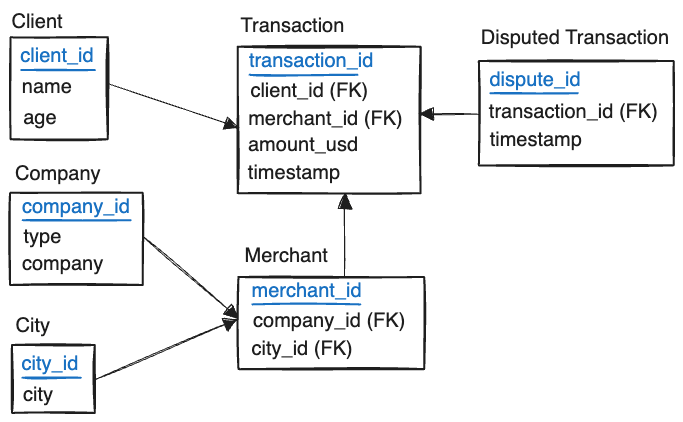
The primary table of interest is the transactions table, which contains records of all the transactions made by a client with a particular merchant. A merchant is a store or a business that provides goods or services. The disputes table contains records of all the disputed transactions, marked after the fact and stored in a separate table.

When considering questions about disputed transactions, aggregation queries are not enough. We need to study the paths between the clients, merchants and transactions. This is where a graph database like Kùzu is very handy. The data model used by Kùzu is a structured property graph model, allowing us to capture the relationships between entities in a more natural way, for specific query workloads such as this one.

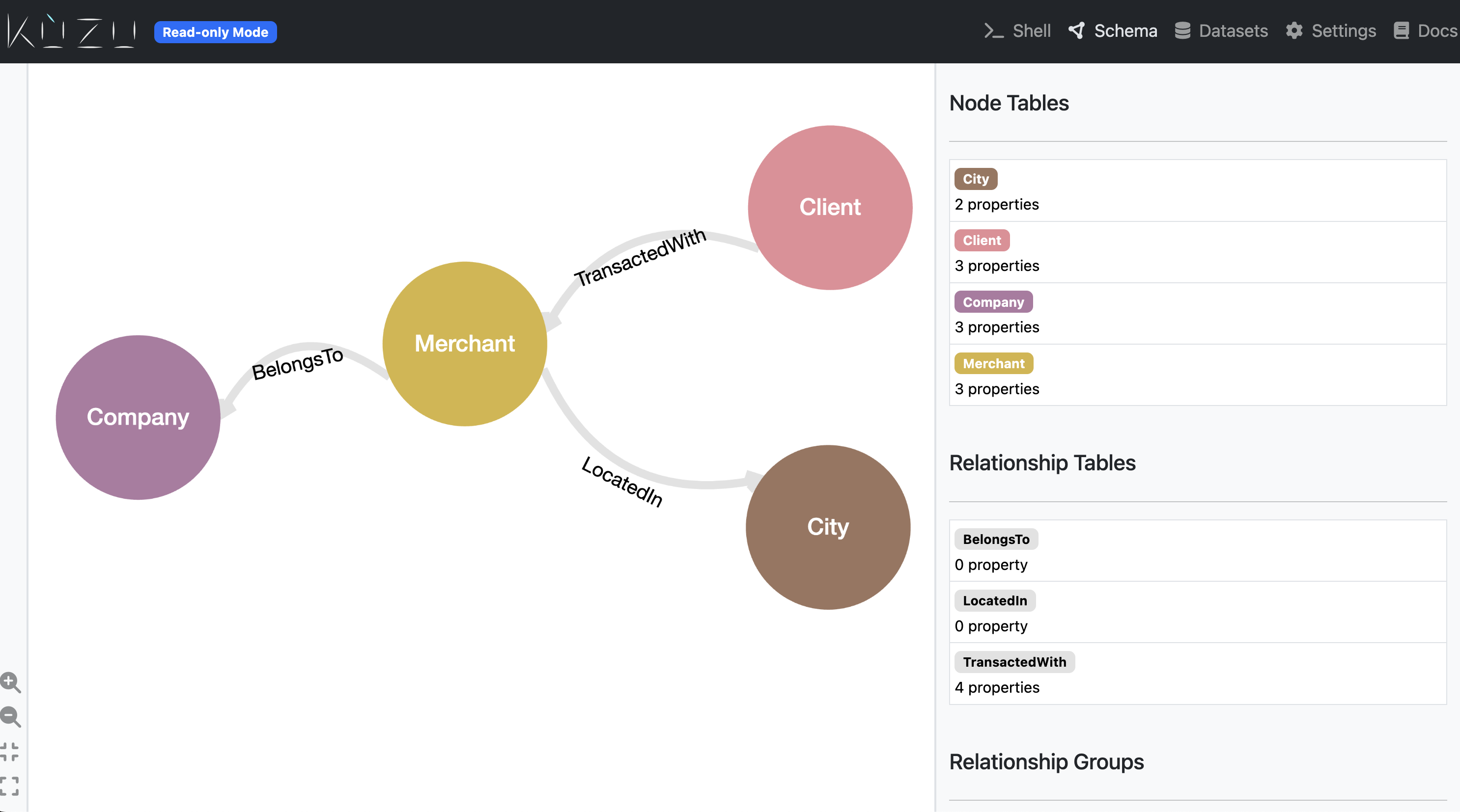
Graph schema

The following graph schema makes sense for our dataset:

The transactions are modelled as edges, with an is_disputed property to indicate whether a transaction is disputed or not. This simplifies the kinds of queries we need to write, and is sufficient for our initial analysis.

Inserting data into Kùzu

The previous post went into the data transformation and ETL aspects, so we won’t go over that here. In a nutshell, the following input files exist in CSV format that need to be inserted into Kùzu:

.
├── data
│   ├── node
│   │   ├── client.csv
│   │   ├── city.csv
│   │   ├── company.csv
│   │   ├── merchant.csv
│   │   └── disputed_transactions.csv
│   └── rel
│       ├── belongs_to.csv
│       ├── located_in.csv
│       └── transacted_with.csv
└── load_data.py

The script load_data.py reads the CSV files and inserts the data into Kùzu using the Python API. The result of running this script is a graph whose schema matches that shown in the sketch above.

Exploratory data analysis

Once the data is loaded into Kùzu, it’s very simple to begin exploring the data using Cypher queries in one of three ways: i) using a Kùzu CLI shell, ii) using a Jupyter notebook, and iii) using the Kùzu Explorer UI. Because the goal of this exercise is to perform exploratory data analysis on the graph, we’ll Kùzu Explorer to visualize the graph and run Cypher queries.

MATCH (c:Client) RETURN COUNT(c) AS numClients

numClients
100

MATCH (m:Merchant) RETURN COUNT(m) AS numMerchants

numMerchants
100

MATCH (:Client)-[t:TransactedWith]->(:Merchant)
RETURN COUNT(t) AS numTransactions

numTransactions
1100

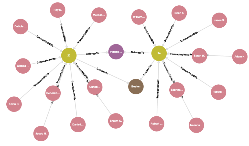
The dataset contains 1,000 clients who made 1,100 transactions with 100 merchants. We can visualize the transactions with a particular merchant at a particular city and belonging to a particular company using the following query:

MATCH (c:Client)-[t:TransactedWith]->(m:Merchant)-[b:BelongsTo]->(co:Company)
MATCH (m)-[l:LocatedIn]->(ci:City {city: "Boston"})
WHERE co.company = "Panera Bread"
RETURN * LIMIT 25;

The dataset contains two merchants belonging to Panera Bread in the city of Boston.

Study disputed transactions

The dataset becomes more interesting when we begin studying disputed transactions. Not all disputed transactions are fraudulent, and so a simple aggregation query won’t reveal many insights. We can begin by isolating only the vicinity of the disputed transactions of the graph by specifying the boolean relationship property is_disputed and then adding a subsequent MATCH statement to find the other merchants with whom clients reported disputed transactions.

MATCH (c:Client)-[t:TransactedWith]->(m:Merchant)
MATCH (c)-[t2:TransactedWith]->(m2:Merchant)
WHERE t.is_disputed = true
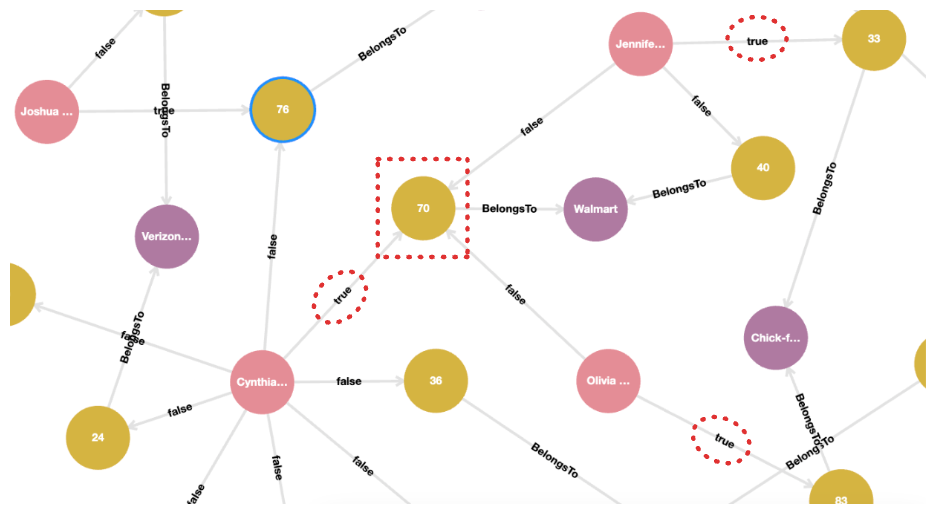
RETURN * LIMIT 25;

When running this query in Kùzu Explorer, we can customize the edge properties displayed in the graph visualization. In the following image, we mark the TransactedWith edges with the boolean value of the is_disputed property from the data. Only a small fraction of these transactions have the is_disputed property marked as true.

It can be seen that certain clients interacted with multiple merchants, some of which form a cluster. In other cases, nodes in the vicinity of a disputed transaction have no common paths with the larger graph, resulting in a disjoint subgraph. Fraud is less likely in the latter case, because a fraudster would likely have interacted with multiple clients that are part of a cluster sharing common merchants.

The list of client names who reported disputed transactions can be listed as follows:

MATCH (c:Client)-[t:TransactedWith]->(m:Merchant)
WHERE t.is_disputed = true
RETURN c.name AS name, t.timestamp AS transactionTime;

name	transactionTime
Joshua T.	2023-11-21T16:54:30Z
Jennifer Y.	2023-12-24T17:39:33Z
Brandon T.	2023-08-04T18:21:27Z
Cynthia J.	2023-12-24T02:49:31Z
Olivia C.	2023-12-27T04:23:04Z

Depending on the dataset, the time stamps of the disputed transactions in comparison to the timestamp of the transaction itself, could yield additional insights. The power of a graph structure is that it allows us to isolate substructures of interest based on the connected nature of the data.

The aim of the next query is to find the city in which the most disputed transactions occurred, and also to which companies the merchants processing these transactions belonged to.

MATCH (c:Client)-[t:TransactedWith]->(:Merchant)
WHERE t.is_disputed = true
WITH c
MATCH (c)-[t2:TransactedWith*..2]->(m:Merchant)-[:BelongsTo]->(co:Company)
WITH c, m, co
MATCH (m)-[:LocatedIn]->(ci:City)
RETURN
    m.merchant_id AS merchantID,
    ci.city AS city,
    co.company AS company,
    COLLECT(c.name) AS clients,
    COUNT(c) AS counts
ORDER BY counts DESC LIMIT 3;

merchantID	city	company	clients	counts
70	Boston	Walmart	["Olivia C.","Jennifer Y.","Cynthia J."]	3
76	San Francisco	Panera Bread	["Joshua T.","Cynthia J."]	2
51	Chicago	AT&T	["Cynthia J.","Cynthia J."]	2

It can be seen that the clients Olivia, Cynthia and Jennifer all reported disputed transactions in a particular merchant location in Boston that belongs to the company Walmart. The query above returned the names of the clients, but in a larger dataset it makes sense to return the number of clients instead.

When viewed visually, these results can be quite powerful. The following image shows result from above, as seen in Kùzu Explorer.

If we simply look at aggregates based on the company and merchant, we see that the clients Olivia, Jennifer and Cynthia from the previous query each reported disputed transactions in different merchant locations. However, they all had a common merchant in Boston (ID 70) belonging to Walmart, that they all made transactions within a plausible time window. This could indicate that this particular merchant, located in Boston, could be a source of fraud.

Graph algorithms

Kùzu is well-integrated with the PyData ecosystem, including PyTorch Geometric, Pandas, and NetworkX, a popular Python library for network analysis. Because Kùzu is an embedded graph database, it runs in-process with a Python application, so it’s simple to isolate a subgraph of interest via Cypher and convert it to a NetworkX directed graph (DiGraph) for further analysis.

Weakly connected components

A weakly connected component is a maximal subgraph in which there is a path between any two nodes, ignoring the direction of the edges. In the context of our subgraph of clients, merchants and the vicinity of disputed transactions, we can use this algorithm to isolate the disjoint subgraphs that we saw in the visualization earlier.

We first isolate the subgraph of clients, merchants and transactions in the vicinity of disputed transactions as follows:

import kuzu
import networkx as nx

db = kuzu.Database("./transaction_db")
conn = kuzu.Connection(db)

# Isolate the subgraph of interest
disputed_vicinity = conn.execute(
    """
    MATCH (c1:Client)-[t1:TransactedWith]->(m:Merchant)<-[t2:TransactedWith]-(c2:Client)
    WHERE t1.is_disputed = true
    RETURN *;
    """
)

# Convert to networkx DiGraph
G1 = clients.get_as_networkx(directed=True)

For every client that reported a disputed transaction, we isolate the subgraph of all the clients who interacted with these same merchants, as well as others. Running the weakly connected components algorithm will first inform us whether the vicinity of disputed transactions is a single connected component or not.

num_weakly_connected_components = nx.number_weakly_connected_components(G1)
print(num_weakly_connected_components)

# Output
2

We obtain 2 weakly connected components, indicating that there are disjoint components in the disputed transactions subgraph.

To see which clients/merchants are in each weakly connected component, we can run the following:

weakly_connected_components = list(nx.weakly_connected_components(G2))

print(len(weakly_connected_components[0]))
print(len(weakly_connected_components[1]))

# Output
52
9

The first cluster of clients and merchants contains 52 nodes, while the second cluster contains 9 nodes. This helps narrow down on a transaction subgraph that has a greater degree of connectivity.

Closeness centrality

Centrality algorithms are among the most commonly used algorithms in graph data science. At a high-level, centrality algorithms are used to identify “important” nodes - specifically, nodes that serve the role of connecting many other nodes in the graph. Suppose the owner of our transaction graph is an e-commerce company, and that the company wants to promote its “important merchants” to attract more customers to its network. Centrality metrics, similar to the popular PageRank metric, are concrete ways to order nodes in terms of “importance”.

Closeness centrality² measures how close a node n is to all other nodes by calculating the average of the shortest path length from n to every other node in the graph. For this example, we will first isolate the full subgraph of all clients, merchants and transactions, not just those in the vicinity of disputed transactions.

subgraph = conn.execute(
    """
    MATCH (c:Client)-[t:TransactedWith]->(m:Merchant)
    RETURN *;
    """
)

# Convert to networkx DiGraph
G2 = subgraph.get_as_networkx(directed=True)

closeness_centrality_result = list(nx.closeness_centrality(G1).items())
closeness_centrality_result.sort(key=lambda x: x[1], reverse=True)
print(closeness_centrality_result[:5])

The top 5 nodes with the highest closeness centrality are shown below:

[('Merchant_35', 0.028),
 ('Merchant_56', 0.02666666666666667),
 ('Merchant_38', 0.025333333333333333),
 ('Merchant_66', 0.025333333333333333),
 ('Merchant_96', 0.024)]

The scores indicate that the merchant with ID 35 is the most central node in the subgraph, i.e., it’s on average the closest to other nodes in the graph as a lot of paths go through it. Pandas makes this process very convenient.

import pandas as pd

df = pd.DataFrame(closeness_centrality_result, columns=["node_id", "closeness_centrality"])
df = df[df["node_id"].str.startswith("Merchant_")]
df["node_id"] = df["node_id"].str.replace("Merchant_", "").astype(int)
df = df.sort_values(by="closeness_centrality", ascending=False).reset_index(drop=True)
print(df.head(5))

node_id	closeness_centrality
35	0.028000
56	0.026667
38	0.025333
66	0.025333
96	0.024000

Once we have the Pandas DataFrame, it’s trivial to write a function that can modify the existing Merchant node table and add the closeness centrality scores back to the graph. Kùzu’s Python API has a native scan feature that can directly read from Pandas DataFrames in a zero-copy manner.

Note that we first alter the original node table schema to add a new column for the closeness centrality scores. We then use the LOAD FROM command to read the Pandas DataFrame into the graph.

try:
    # Alter original node table schema to add degree centrality
    conn.execute('ALTER TABLE Merchant ADD closeness_centrality DOUBLE DEFAULT 0.0')
except RuntimeError:
    # If the column already exists, do nothing
    pass
# Read degree centrality to graph
conn.execute(
    """
    LOAD FROM df
    MERGE (m:Merchant {merchant_id: node_id})
    ON MATCH SET m.closeness_centrality = closeness_centrality
    RETURN *;
    """
)

Applying a similar process to the client nodes (via other centrality algorithms like degree centrality) can help us use these scores in downstream machine learning models, or to inform further decisions.

Conclusions

Hopefully, this post has given you a good idea of how to use Kùzu to effectively model and analyze your data via a combination of Cypher and graph algorithms. It’s worth keeping in mind that Graph data science, just like conventional data science, is an iterative process. The ability to think of structured data (in tables) as graphs helps us rapidly isolate interesting subsets of the data, run graph algorithms and visualize substructures, making these powerful tools in the data scientist’s toolkit.

Kùzu’s in-process architecture makes it very friendly towards these sorts of workflows without the data scientist having to worry about servers or managing infrastructure. Data can be conveniently read into Kùzu from a variety of sources, including relational databases, CSV or parquet files, or DataFrames. Future versions of Kùzu will support more convenience features, such as the ability to natively scan PostgreSQL tables, as well as native support for Arrow tables.

In summary, the interoperability of an embedded graph database with popular Python libraries like NetworkX and Pandas makes Kùzu a powerful tool for graph data science. If you have data of a similar nature in the form of relational tables, we highly recommend you to think about whether your use case can benefit from graph data models. If so, give Kùzu a try and reach out to us on Discord with your experiences and feedback!

Code

The code to reproduce the workflow shown in this post can be found in the graphdb-demo repository. It uses Kùzu’s Python API, but you are welcome to use the client API of your choice.

Further reading

Footnotes

1. Graph Powered Machine Learning, Ch. 2, By Alessandro Negro, Manning Publications, 2021. ↩

2. When is the Closeness Centrality Algorithm best applied? [blog post] (https://www.graphable.ai/blog/closeness-centrality-algorithm/), By Fatima Rubio, Graphable ↩