Factorization and great ideas from database theory

CEO of Kùzu Inc. & Associate Prof. at UWaterloo
Many of the core principles of how to develop DBMSs are well understood. For example, a very good query compilation paradigm is to map high-level queries to a logical plan of relational operators, then optimize this plan, and then further map it to an executable code often in the form of a physical query plan. Similarly, if you want updates to a DBMS to be atomic and durable, a good paradigm is to use a write-ahead log that serves as a source of truth and can be used to undo or redo operations. Many systems adopt such common wisdom paradigms. As core DBMS researcher, once in a while however, you run into a very simple idea that deviates from the norm that gets you very excited. Today, I want to write about one such idea called factorization.
TL;DR: The key takeaways are:
-
Overview of Factorization & Why Every GDBMS Must Adopt It: Factorization is a compression technique to compress the intermediate results that query processors generate when evaluating many-to-many (m-n) joins. Factorization can compress an intermediate result size exponentially in the number m-n joins in the query.
-
Example Benefits of Factorization: Benefits of keeping intermediate results smaller reduces the computation processors perform on many queries. Examples include reducing copies by keeping the output data size small, reducing filter and expression evaluation computations exponentially, and performing very fast aggregations.
-
How Kuzu Implements Factorization: Kuzu’s query processor is designed to achieve 3 design goals: (i) factorize intermediate results; (ii) always perform sequential scans of database files; and (iii) avoid scanning large chunks of database files when possible. In addition, the processor is vectorized as in modern columnar DBMSs. These design goals are achieved by passing multiple factorized vectors between each other and using modified HashJoin operators that do sideways information passing to avoid scans of entire files.
This is a rather technical and long blog post and will appeal more to people who are interested in internals of DBMSs. It’s about a technique that’s quite dear to my heart called factorization, which is a very simple data compression technique. Probably all compression techniques you know are designed to compress database files that are stored on disk. Think of run-length encoding, dictionary compression, or bitpacking. In contrast, you can’t use factorization to compress your raw database files. Factorization has a very unique property: it is designed to compress the intermediate data that are generated when query processors of DBMSs evaluate many-to-many (m-n) growing joins. If you have read my previous blog, efficiently handling m-n joins was one of the items on my list of properties that competent GDBMSs should excel in. This is because the workloads of GDBMSs commonly contain m-n joins across node records. Each user in a social network or an account in a financial transaction network or will have thousands of connections and if you want a GDBMS to find patterns on your graphs, you are asking queries with m-n joins. Factorization is directly designed for these workloads and because of that every competent GDBMS must develop a factorized query processor. In fact, if I were to try to write a new analytical RDBMS, I would probably also integrate factorization into it.
This post forms the 2nd part of my 3-part posts on the contents of our CIDR paper where we introduced Kuzu. The 3rd piece will be on another technique called worst-case optimal join algorithms, which is also designed for a specific class of m-n joins. Both in this post and the next, I have two goals. First is to try to articulate these techniques using a language that is accessible to general software engineers. Second, is to make people appreciate the role of pen-and-paper theory in advancing the field of DBMSs. Both of these techniques were first articulated in a series of purely theoretical papers which gave excellent practical advice on how to improve DBMS performance. Credit goes to the great theoreticians who pioneered these techniques whom I will cite in these posts. Their work should be highly appreciated.
A Quick Background: Traditional Query Processing Using Flat Tuples
Here is a short background on the basics of
query processors before I explain factorization. If you know about
query plans and how to interpret them,
you can skip to here after reading
my running example.
Consider a database of Account node and Transfer edge records below.
The two Accounts with accID fields L1 and L2 are owned by Liz and
each have 100 incoming and 100 outgoing Transfer edges.
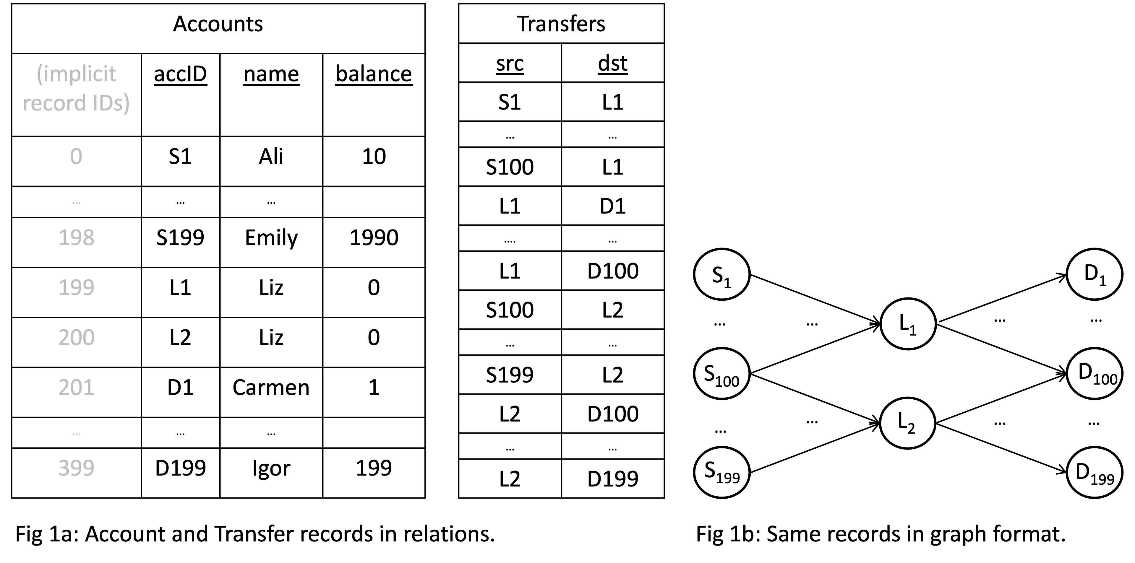
Now consider a 2-hop path query in Cypher returning the accID’s of source and destinations of money flows Liz’s accounts are facilitating:
MATCH (a:Account)-[t1:Transfer]->(b:Account)-[t2:Transfer]->(c:Account)
WHERE b.name = 'Liz'
RETURN a.accID, c.accID
Here’s the SQL version of the query if you modeled your records as relations. Same query different syntax:
SELECT a.accID, c.accID
FROM Account a, Transfer t1, Account b, Transfer t2, Account c
WHERE b.name = 'Liz' AND
      t1.src = a.accID AND t1.dst = b.accID AND
      t2.src = b.accID AND t2.dst = c.accID
A standard query plan for this query is shown on the left in Fig. 2. The plan contains some Scan operators to scan the raw node or edge records (edges could be scanned from a join index) and some hash join operators to perform the joins, and a final projection operator. In some GDBMSs, you might see “linear plans” that look as in Fig. 3.
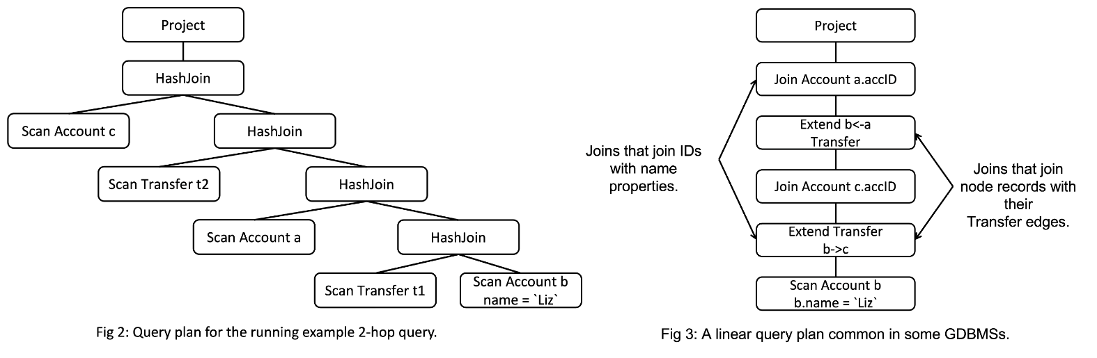
The linear plan is from our previous GraphflowDB system. Here you are seeing an operator called Extend, which joins node records with their Transfer relationships to read the system-level IDs of the neighbors of those node records. Following the Extend is another Join operator to join the accID properties of those neighbors (specifically c.accID and a.accID). In Neo4j, you’ll instead see an Expand(All) operator, which does the Extend+Join in GraphflowDB in a single operator1. For very good reasons we removed these Extend/Expand type operators in Kuzu. I will come back to this.
The interpretation of plans is that tuples are flowing from the bottom to top and each operator will take in sets of tuples and produce sets of tuples (in a pipelined fashion). The key motivation for factorization is that what flows between operators are flat tuples. When the joins are m-n, this leads to many data repetitions, which one way or another leads to repeated computation in the operators. For example, the final projection operator in our example would take the table shown in Figure 4 (left).
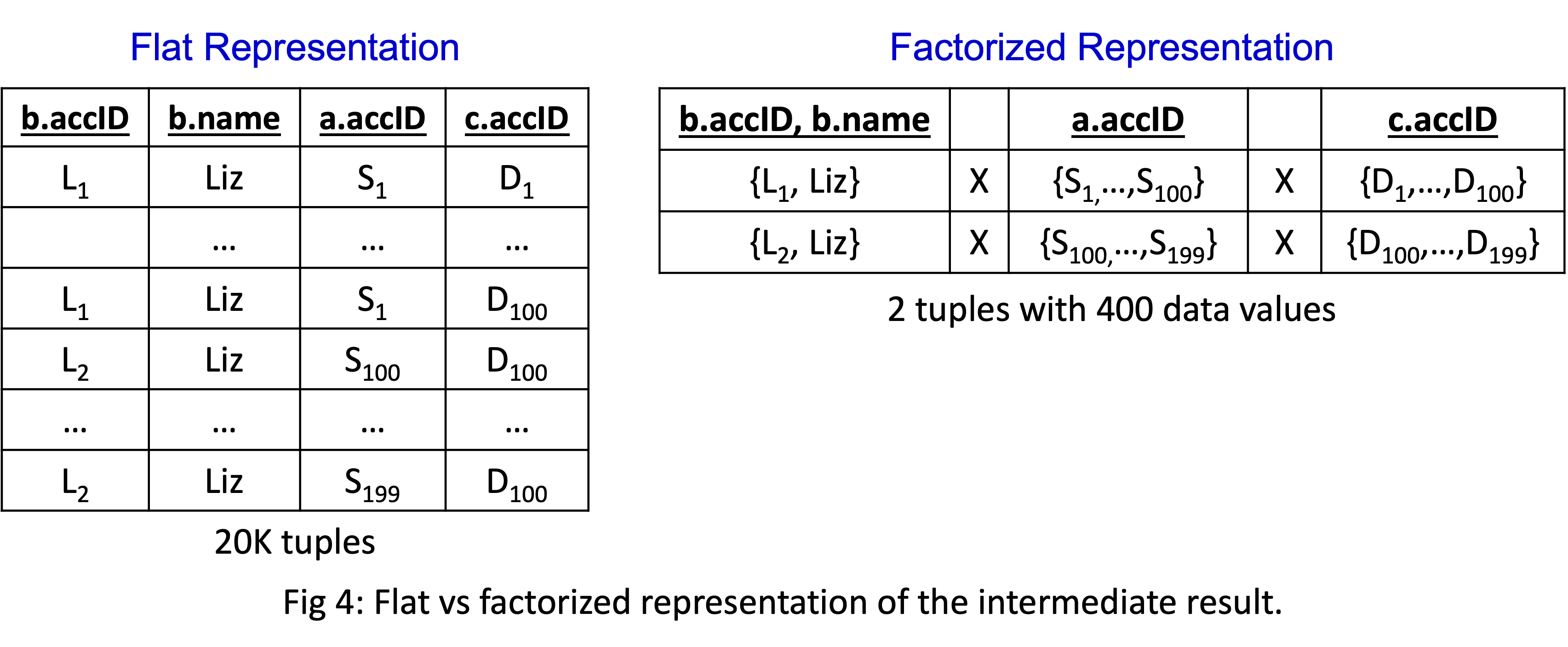
There are 20K tuples in the flat representation because both L1 and L2 are part of 100 incoming x 100 outgoing=10K many 2-paths. Notice the many repetitions in this relation: L1, L2, or Liz values, or the values in a.accID and c.accID. What gets replicated may change across systems. Some may replicate the actual values, some may replicate indices where these values are stored but overall exactly 20K tuples would be generated. This redundancy leads to redundant computation here and there during query processing.
Factorization In a Nutshell
Factorization addresses exactly this problem. The core reason for the redundancy
is this observation: given a fixed b value, all a’s and c’s are conditionally independent.
More concretely, once b is bound to node L1, each incoming neighbor a for L1 will join
with each outgoing neighbor c of L1. If you took the first standard undergraduate course in DBMSs at a university
and you covered the theory of normalization, this is what is
called a multi-valued dependency
in relations. Factorization exploits such dependencies to compress
relations using Cartesian products.
Above in Figure 4 (right),
I’m showing the same 20K tuples in a factorized format using only 400 values
(so 2*(100 + 100) instead of 2*100*100 values).
That’s it! That’s the core of the idea! Now of course, this simple observation leads to a ton of hard and non-obvious questions that the entire theory on factorization answers. For example, given a query, what are the “factorization structures”, i.e., the Cartesian product structures that can be used to compress it? Consider a simple query that counts the number of paths that are slightly longer:
MATCH (a:Account)-[:Wire]->(b:Account)-[:Deposit]>(c:Account)-[:ETransfer]->(d:Account)
RETURN count(*)
Should you condition on b and factor out a’s from (c, d)‘s or condition on c and factor out (a, b)‘s from d’s? Or you could condition on (b, c) and factor out (a)‘s from (d)‘s? To make a choice, a system has to reason about the number of Wire, Deposit, and ETransfer records in the database. How much and on which queries can you benefit from factorization? The theoretical questions are endless. The theory of factorization develops the formal foundation so that such questions can be answered and provides principled first answers to these questions. Dan Olteanu and his colleagues, who lead this field, recently won the ICDT test of time award for their work on factorization. ICDT is one of the two main academic venues for theoretical work on DBMSs.
But let’s take a step back and appreciate this theory because it gives an excellent advice to system developers: factorize your intermediate results if your queries contain many-to-many joins! Recall that GDBMSs most commonly evaluate many-to-many joins. So hence my point that GDBMSs should develop factorized query processors. The great thing this theory shows us is that this can all be done by static analysis of the query during compilation time by only inspecting the dependencies between variables in the query! I won’t cover the exact rules but at least in my running example, I hope it’s clear that because there is no predicate between a’s and c’s, once b is fixed, we can factor out a’s from c’s.
Examples When Factorization Significantly Benefits:
Factorized intermediate relations can be exponentially smaller (in terms of the number of joins in the query) than their flat versions, which can yield orders of magnitude speed ups in query performance for many different reasons. I will discuss three most obvious ones.
Less Data Copies/Movement
The most obvious benefit is that factorization reduces
the amount of data copied between buffers used by operators
during processing and to final QueryResult structure
that the application gets access to. For example, a very cool feature of Kuzu
is that it keeps final outputs in factorized format in its QueryResult class and
enumerates them one by one only when the user starts calling QueryResult::getNext()
to read the tuples.
In our running example, throughout processing Kuzu would do copies of
400 data values roughly instead of 20K to produce its QueryResult.
Needless to say, I could have picked a more exaggerated query, say a “star” query
with 6 relationships, and arbitrarily increased the difference in the copies done
between a flat vs factorized processor.
Fewer Predicate and Expression Evaluations
Factorization can also reduce the amount of predicate or expression executions the system performs. Suppose we modify our 2-hop query a bit and put two additional filters on the query:
MATCH (a:Account)-[e1:Transfer]->(b:Account)-[e2:Transfer]->(c:Account)
WHERE b.name = 'Liz' AND a.balance > b.balance AND c.balance > b.balance
RETURN *
I’m omitting a plan for this query but a common plan would extend the plan in Figure 2 (or 3) above
to also scan the balance properties and to run two filter operations:
(i) above the join that joins a’s and b’s,
to run the predicate a.balance > b.balance; (ii) after the final join in Figure 2
to run the predicate c.balance > b.balance. Suppose the first filter did not eliminate any tuples.
Then, a flat processor would evaluate 20K filter executions in the second filter.
In contrast, the input to the second filter operator in a factorized processor
would be the 2 factorized tuples
shown in Figure 4 (right) but extended with balance properties
on a, b, and c’s. Therefore there would be only 200 filter executions: (i)
for the first factorized tuple, there are only
100 comparisons to execute c.balance > b.balance since b is matched to a single
value and there are 100 c values.; (ii) similarly for the 2nd factorized tuple.
We can obtain similar benefits when running other expressions.
Aggregations
This is perhaps where factorization yields largest benefits.
One can perform several aggregations directly on factorized tuples using
algebraic properties of several aggregation functions. Let’s
for instance modify our above query to a count(*) query: Find the number of 2-paths that Liz is
facilitating. A factorized processor can simply count that there are 100 x 100 flat tuples in the first
factorized tuple and similarly in the second one to compute that the answer is 20K.
Or consider doing min/max aggregation on factorized variables:
MATCH (a:Account)-[e1:Transfer]->(b:Account)-[e2:Transfer]->(c:Account)
WHERE b.accID = 'L1'
RETURN max(a.balance), min(c.balance)
This is asking: find the 2-path money flow that Liz’s L1 account facilitates from the highest to lowest balance accounts (and only print the balances). If a processor processes the 10K 2-paths that L1 is part of in factorized form, then the processor can compute the max and min aggregations with only 100 comparisons each (instead of 10K comparisons each).
In short, the benefits of factorizing intermediate results just reduces computation and data copies here and there in many cases. You can try some of these queries on Kuzu and compare its performance on large datasets with non-factorized systems.
How Does Kuzu Perform Factorized Query Processing?
The rest will be even more technical and forms part of the technical meat of our CIDR paper; so continue reading if you are interested in database implementations. When designing the query processor of Kuzu, we had 3 design goals:
- Factorize intermediate growing join results.
- Always perform sequential scans of database files from disk.
- When possible avoid scanning entire database files from disk.
3rd design goal requires some motivation, which I will provide below. Let’s go one by one.
1. Factorization
Kuzu has a vectorized query processor, which is the common wisdom in analytical read-optimized systems.
Vectorization, in the context of DBMS query processors
refers to the design where operators pass a set of tuples, 1024 or 2048,
between each other during processing2. Existing vectorized query processors (in fact
processors of all systems I’m aware of) pass a single vector of flat tuples.
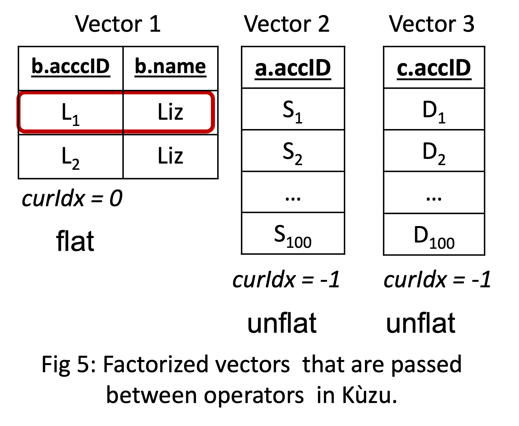
Instead, Kuzu’s operators pass (possibly) multiple factorized vectors of tuples
between each other. Each vector can either be flat and represent a single value or
unflat and represent a set of values, which is marked in a field called curIdx
associated with each vector.
For example, the first 10K tuples from my running example would be represented
with 3 factorized vectors as on the left and would be passed to the final projection
in the query plan in Figure 2.
The interpretation is this: what is passed is the Cartesian product of all sets of
tuples in those vectors. Operators know during compilation time how many vector
groups they will take in and how many they will output. Importantly, we still
do vectorized processing, i.e., each primitive operator operates on a vector of values
inside tight for loops.
Credit where credit’s due: this simple-to-implement design was proposed
by my PhD student Amine Mhedhbi with some feedback from
me and my ex-Master’s student
Pranjal Gupta
and Xiyang Feng,
who is now a core developer of Kuzu.
And we directly adopted it in Kuzu. Amine has continued doing other excellent
work on factorization, which we have not yet integrated, and you
will need to wait until his PhD thesis is out.
2. Ensuring Sequential Scans
I already told you above that Extend/Expand type join operators lead to non-sequential scans of database files. These operators are not robust and if you are developing a disk-based system: non-sequential scans will kill you on many queries. That’s a mistake. Instead, Kuzu uses (modified) HashJoins which are much more robust. HashJoins do not perform any scans as part of the actual join computation so if the down stream scans are sequential, you get sequential scans. I’ll give a simulation momentarily.
3. Avoiding Full Scans of Database Files
Although I don’t like Extend/Expand-type join operators, they have a performance advantage. Suppose you had a simple 1-hop query that only asked for the names of accounts that Liz’s L1 account has transfered money to:
MATCH (a:Account)-[:Transfer]->(b:Account)
WHERE a.accID = 'L1'
RETURN b.name
Suppose your database has billions of transfers but L1 has made only 3 transfers to accounts with system-level record/node IDs: 107, 5, and 15. Then if you had a linear plan like I showed in Figure 3, then an Extend/Expand-type operator could read these system-level IDs and then only scan the name properties of these 3 nodes, avoiding the full scan of the names of all Accounts. If your query needs to read neighborhoods of millions of nodes, this type of computation that “reads the properties of each node’s neighbors” will degrade very quickly because: (i) each neighborhood of each node will require reading different parts of the disk files that store those properties; and (ii) the system might repeatedly read the same properties over and over from disk, as nodes share neighbors. Instead, you want to read all of the properties and create a hash table and read those properties from memory. However, if your query is accessing the neighborhoods of a few nodes, then avoiding the scan of entire database file is an advantage. In Kuzu, we wanted to use HashJoins but we also wanted a mechanism to scan only the necessary parts of database files. We do this through a technique called sideways information passing3. I’ll simulate this below.
A Simple Simulation
For simplicity, we’ll work on a simpler 1-hop query, so the benefits of factorization will not be impressive but it will allow me to explain an entire query processing pipeline. Consider this count(*) query that counts the number of transfers the L1 account has made:
MATCH (a:Account)-[t1:Transfer]->(b:Account)
WHERE a.accID = L1
RETURN count(*)
An annotated query plan we generate is shown below. The figure shows step by step the computation that will be performed and the data that will be passed between operators. For this simulation, I am assuming that the record/nodeIDs of Accounts are as in Figure 1a above.

- A Scan operator will scan the accId column and find the records of
nodes with
accID=L1. There is only 1 tuple(199, Liz)that will be output. - This tuple will passed to HashJoin’s build side, which will create a hash table from it.
- At this point the processor knows exactly the IDs of nodes, whose Transfer edges need to be scanned on the probe side: only the edges of node with ID 199! This is where we do sideways information passing. Specifically, the HashJoin constructs and passes a “nodeID filter” (effectively a bitmap) to the probe side Scan operator. Here, I’m assuming the database has 1M Accounts but as you can see only the position 199 is 1 and others are 0.
- The probe-side Scan uses the filter to only scan
the edges of 199 and avoids
scanning the entire Transfers file.
Since Kuzu is a GDBMS, we store the edges of nodes (and their properties)
in a graph-optimized format called CSR.
Importantly, all of the edges of 199 are stored consecutively and we output them in factorized format as:
[(199) X {201, 202, ..., 300}]. - Next step can be skipped in an optimized system but currently we will probe the
[(199) X {201, 202, ..., 300}]tuple in the hash table and produce[(199, L1) X {201, 202, ..., 300}], which is passed to the final aggregation operator. - The aggregation operator counts that there are 100 “flat” tuples in
[(199, L1) X {201, 202, ..., 300}], simply by inspecting the size of the 2nd vector{201, 202, ..., 300}in the tuple.
As you see the processing was factorized, we only did sequential scans but we also avoided scanning the entire Transfer database file, achieving our 3 design goals. This is a simplifid example and there are many queries that are more complex and where we have more advanced modified hash join operators. But the simulation presents all core techniques in the system. You can read our CIDR paper if you are curious about the details!
Example Experiment
How does it all perform? Quite well! Specifically this type of processing is quite robust. Here’s an experiment from our CIDR paper to give a sense of the behavior of using modified hash joins and factorization on a micro benchmark query. This query does a 2-hop query with aggregations on every node variable. This is on an LDBC social network benchmark (SNB) dataset at scale factor 100 (so ~100GB of database). LDBC SNB models a social network where user post comments and react to these comments.
MATCH (a:Comment)<-[:Likes]-(b:Person)-[:Likes]->(c:Comment)
WHERE b.ID < X
RETURN min(a.ID), min(b.ID), min(c.ID)
Needless to say, we are picking this as it is a simple query that can demonstrate the benefits of all of the 3 techniques above. Also needless to say, we could have exaggerated the benefits by picking larger stars or branched tree patterns but this will do. In the experiment we are changing the selectivity of the predicate on the middle node, which changes the output size. What we will compare is the behavior of Kuzu, which integrates the 3 techniques above with (i) Kuzu-Extend: A configuration of Kuzu that uses factorization but instead of our modified HashJoins uses an Extend-like operator; and (ii) Umbra4, which represents the state of the art RDBMS. Umbra is as fast as existing RDBMSs get. It probably integrates every known low-level performance technique in the field. Umbra however does not do factorization or have a mechanism to avoid scanning entire database files, so we expect it to perform poorly on the above query.
Here’s the performance table.
| Selectivity | Kuzu | Kuzu-Extend | Umbra |
|---|---|---|---|
| 0.01% | 0.33 | 0.01s | 1.90s |
| 0.1% | 0.41s | 0.11s | 4.05s |
| 1% | 0.96s | 1.04s | 12.30s |
| 10% | 3.89s | 10.39s | 230.35s |
| 100% | 31.98s | 92.35s | TO |
When the selectivity is very low, Extend-like operators + factorization do quite well because they don’t yet suffer much from non-sequential scans and they avoid several overheads of our modified hash joins: no hash table creation and no semijoin filter mask creation. But they are not robust and degrade quickly. We can also see that even if you’re Umbra, without factorization or a mechanism to avoid scanning entire files, you will not perform very well on these queries with m-n joins (even if there is only 2 of them here). We conducted several other experiments all demonstrating the robustness and scalability of factorized processing using modified hash join operators. I won’t cover them but they are all in our CIDR paper.
Final marks:
I am convinced that modern GDBMSs have to be factorized systems to remain competitive in performance. If your system assumes that most joins will be growing, factorization is one of a handful of modern technique for such workloads whose principles are relatively well understood and one can actually implement in a system. I am sure different factorized query processors will be proposed as more people attempt at it. I was happy to see in CIDR that at least 2 systems gurus told me they want to integrate factorization into their systems. If someone proposes a technique that can on some queries lead to exponential computation reductions even in a pen-and-paper theory, it is a good sign that for many queries it can make the difference between a system timing out vs providing an actual answer.
Finally there is much more on the theory of factorization, which I did not cover. From my side, most interestingly, there are even more compressed ways to represent the intermediate results than the vanilla Cartesian product scheme I covered in this post. Just to raise some curiosity, what I have in mind is called d-representations but that will have to wait for another time. For now, I invite you to check our performance out on large queries and let us know if we are slow on some queries! The Kuzu team says hi (👋 🙋♀️ 🙋🏽) and is at your service to fix all performance bugs as we continue implementing the system! My next post will be about the novel worst-case optimal join algorithms, which emerged from another theoretical insight on m-n joins! Take care until then!
Footnotes
-
If you come from a very graph-focused background and/or exposed to a ton of GDBMS marketing, you might have a strong reaction to my statement that all I’m showing are standard plans that do joins. Maybe you expected to see graph-specific operators, such as a BFS or a DFS operator because the data is a graph. Or maybe someone even dared to tell you that GDBMSs don’t do joins but they do traversals. Stuff like that. These word tricks and confusing jargon really has to stop and helps no one. If joins are in the nature of the computation you are asking a DBMSs to do, calling it something else won’t change the nature of the computation. Joins are joins. Every DBMSs needs to join their records with each other. ↩
-
Vectorization emerged as a design in the context of columnar RDBMSs, which are analytical systems, about 15-20 years old. It is still a very good idea. The prior design was to pass a single tuple between operators called Volcano-style tuple-at-a-time processing, which is quite easy to implement, but quite inefficient on modern CPUs. If you have access to the following link, you can read all about it from the pioneers of columnar RDBMSs. ↩
-
Note that GDBMSs are able to avoid scans of entire files because notice that they do the join on internal record/node IDs, which mean something very specific. If a system needs to scan the name property of node with record/node ID 75, it can often arithmetically compute the disk page and offset where this is stored, because record IDs are dense, i.e., start from 0, 1, 2…, and so can serve as pointers if the system’s storage design exploits this. This is what I was referring to as “Predefined/pointer-based joins” in my previous blog post. This is a good feature of GDBMSs that allows them to efficiently evaluate the joins of node records that are happening along the “predefined” edges in the database. I don’t know of a mechanism where RDBMSs can do something similar, unless they develop a mechanism to convert value-based joins to pointer-based joins. See my student Guodong’s work last year in VLDB of how this can be done. In Kuzu, our sideways information passing technique follows Guodong’s design in this work. ↩
-
Umbra is being developed by Thomas Neumann and his group. If Thomas’s name does not ring a bell let me explain his weight in the field like this. As the joke goes, in the field of DBMSs: there are gods at the top, then there is Thomas Neumann, and then other holy people, and then we mere mortals. ↩