
Ever since the birth of database management systems (DBMSs), tabular relations and graphs have been the core data structures used to model application data in two broad classes of systems: relational DBMSs (RDBMS) and graph DBMSs (GDBMS).
In this post, we’ll look at how to transform data that might exist in a typical relational system to a graph and load it into a Kuzu database. The aim of this post and the next one is to showcase “graph thinking”1, where you explore connections in your existing structured data and apply it to potentially uncover new insights.
When are graphs useful?
Enterprise data often exists in the form of relational tables. In an RDBMS, connections between entities are often implicitly defined by the schema of the tables via foreign key constraints. Graphs instead represent records in a more object-oriented manner by explicitly defining entities (or objects) and relationships (or edges) between these entities, offering several benefits:
- A graph data model provides a more natural abstraction to represent indirect or recursive relationships between entities as paths.
- Graph models generally have better support for less-structured or heterogenous data, where objects can be of multiple types or connect to other objects in non-uniform ways. The relational data model on the other hand, requires strict schematization of the data and SQL requires joining records through explicitly named tables.
Query languages over graphs often provide the means to find relationships between nodes without
explicitly naming them, e.g., in Cypher, the (a:Person {name: "Alice})-[]->(b:Person {name:Bob})
pattern will find all possible relationships between nodes with names Alice and Bob. Although SQL is
suitable to express queries for a variety of standard data analytics tasks, it is arguably not as
suitable when it comes to expressing queries with recursive joins or those that describe complex
patterns — they are expressed more naturally as paths or graph patterns. Graph queries
in a well-designed GDBMS like Kuzu contain specialized syntaxes
and operators for these types of query workloads.
For a much more detailed description on the benefits of graph modeling and GDBMSs, see our earlier blog post.
Note
It’s important to understand that data itself doesn’t exist as graphs, tables, arrays and so on. These are just different ways of representing and storing the data. It’s completely up to the developer to choose the right data structure depending on question being answered or the application being developed.
Extract, Transform, Load (ETL)
The dataset we’ll use in this post involves a set of merchants, customers and transactions2. The goal is to study the transactions and their relationships using graph queries.
Relational schema
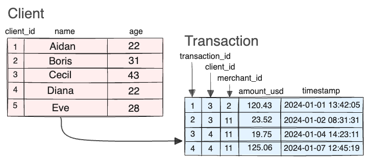
We can imagine this dataset as it exists in a typical relational system. The schema might look something like this:

The client table stores unique client IDs and their metadata. The merchant table stores unique instances of merchants and what parent company they belong to. Transaction data is stored in the transaction table, which shows the transaction ID, the client ID, the merchant ID, the amount of the transaction and when it occurred. Company and city tables exist to store metadata about the parent companies and cities where the merchants are located. The connectivity between the tables is expressed via foreign key constraints.
Graph schema
While the relational schema is useful for rapidly storing transactional data and for performing aggregate queries, it’s not as useful when it comes to answering questions about the relationships in the data. Some such questions are listed below:
- Who are the clients of Company X, i.e., clients who transacted with the merchants of Company X?
- Who are the clients who transacted with at least 2 separate merchants operating in City A?
- Which companies have merchants in City X, City Y and City Z (i.e., in all 3 cities)?
- What connections exist between Client A and Client B (maybe they transacted with the same merchant, or with merchants in the same city, or with merchants belonging to the same company)?
With these questions in mind, we can proceed to sketch the following graph schema, which is a visual representation of a data model that considers how the concepts are connected in the real world.

In the schema above, note how the implicit foreign keys defined in the relational
schema, such as the one between Merchant and City, get explicit names, such as LocatedIn.
Similarly, the two foreign keys in the Transaction relation between Client and Merchant get an
explicit name TransactedWith.
Transforming relational data to graphs
A key feature of Kuzu is that it’s a schema-based graph database, making it highly convenient to read data that already exists in relational systems. Like RDBMSs, Kuzu also relies on strongly-typed values in columns and uses primary key constraints on tables to model the data. The only difference is that Kuzu uses separate node and edge tables, which we’ll show how to create below.
As such, Kuzu can be viewed as a relational system that provides graph modeling capabilities over your tables, allowing you to express graph-based paths and patterns very efficiently in Cypher, the query language implemented by Kuzu.
In this post, for simplicity, we’ll assume that the tables we showed in the relational schema are available
as CSV files in the data directory. The load_data.py script will transform and load the
data into a Kuzu database, while the query.py file will run some simple queries to test that
the load was successful.
.
├── data
│   ├── client.csv
│   ├── city.csv
│   ├── company.csv
│   ├── merchant.csv
│   └── transaction.csv
├── load_data.py
└── query.py
Node tables
The data in the client.csv, city.csv, company.csv and merchant.csv files are already in the
right structure for Kuzu to load them as node tables. You can create the node tables using the
following Cypher queries and run them via the Kuzu CLI, or the client SDK of your choice.
// Client node table
CREATE NODE TABLE Client(
    client_id INT64,
    name STRING,
    age INT64,
    PRIMARY KEY (client_id)
)
// City node table
CREATE NODE TABLE City(
city_id INT64,
city STRING,
PRIMARY KEY (city_id)
)// Company node table
CREATE NODE TABLE Company(
company_id INT64,
type STRING,
company STRING,
PRIMARY KEY (company_id)
)// Merchant node table
CREATE NODE TABLE Merchant(
merchant_id INT64,
company_id INT64,
city_id INT64,
PRIMARY KEY (merchant_id)
)Note that PRIMARY KEY constraints are required on every node table in Kuzu, as they are used to
ensure that edges are always created on unique node pairs. In this case, we use the client_id,
city_id, company_id and merchant_id columns as the primary keys for each respective table.
Edge tables
The graph schema we designed above requires us to transform some of the existing CSV files in order to represent the right columns as edge connections in the graph. We’ll need to create the following files:
transacted_with.csv: connects a client to a merchantbelongs_to.csv: connects a merchant to its parent companylocated_in.csv: connects a merchant to a city
We first define the empty table schemas using the FROM and TO keywords that indicate the
direction of the edge. The names of the tables: TransactedWith, BelongsTo and LocatedIn
are the relationship type.
// TransactedWith edge table
CREATE REL TABLE TransactedWith(
    FROM Client TO Merchant,
    amount_usd FLOAT,
    timestamp TIMESTAMP
)
// BelongsTo edge table
CREATE REL TABLE LocatedIn(FROM Merchant TO City)// LocatedIn edge table
CREATE REL TABLE BelongsTo(FROM Merchant TO Company)In the above code, only TransactedWith edges have properties associated with them, namely the
transaction amount and the timestamp. The other two edges don’t have properties and are simply
used to connect the nodes based on the values that match a primary key constraint.
The data for the edges require minor transformations to the existing CSV files in which the first
and second columns respectively represent the FROM and TO nodes’ primary keys. To help reduce
the amount of custom code you have to write, Kuzu provides convenient APIs to
scan/read from CSV files and to copy data from CSV files to a node or edge table. An example is
shown below.
The transaction.csv file contains the client_id and merchant_id columns, which are the FROM
and TO nodes’ primary keys respectively, but these are not present in the first and second columns
as the edge table requires. To do this, transaction.csv file isn’t loaded as-is, but is instead
transformed into the transacted_with.csv file via the following query.
// Generate `transacted_with.csv` from `transaction.csv`
COPY (
    LOAD FROM 'transaction.csv' (header=true)
    RETURN
        client_id,
        merchant_id,
        amount_usd,
        timestamp
)
TO 'transacted_with.csv';
The example above consists of two subquery blocks: LOAD and COPY. The LOAD block is used to
scan the CSV file, check for headers and data types and return the columns we need. The COPY
block is used to write the results we obtained from the scan to a new file.
We can do the same for the other two edge tables as well.
// Generate `belongs_to.csv` from `merchant.csv`
COPY (
    LOAD FROM 'merchant.csv' (header=true)
    RETURN
        merchant_id,
        company_id
)
TO 'belongs_to.csv';
// Generate `located_in.csv` from `merchant.csv`
COPY (
LOAD FROM 'merchant.csv' (header=true)
RETURN
merchant_id,
city_id
)
TO 'located_in.csv';With all the input files in place, we can now proceed to insert the data and build the graph!
Insert data into Kuzu
Collecting all the above functions, we can write a script that performs the following:
- Transform node/edge tables as needed
- Create the node tables
- Create edge tables
- Load the node tables into the database
- Load the edge tables into the database
In Python, it would look something like this:
// Copy from CSV to node tables
COPY Client FROM 'client.csv' (header=true)
COPY City FROM 'city.csv' (header=true)
COPY Company FROM 'company.csv' (header=true)
COPY Merchant FROM 'merchant.csv' (header=true)

// Copy from CSV to edge tables
COPY TransactedWith FROM 'transacted_with.csv'
COPY BelongsTo FROM 'belongs_to.csv'
COPY LocatedIn FROM 'located_in.csv'
The queries above require that the empty tables were created beforehand. The COPY <edge_table> FROM <file> statement
writes the data into a Kuzu database. Running the queries on an existing database connection
results in the graph being saved to a local directory.
Querying the graph
We then run some simple queries to test that the data was loaded correctly. We can either create a standalone script using the client SDK of your choice, or fire up a Kuzu CLI shell and run some Cypher queries.
The first query finds all the clients who transacted with the merchants of “Starbucks”.
// Q1. Who are the clients that transacted with the merchants of "Starbucks"?
MATCH (c:Client)-[:TransactedWith]->(:Merchant)-[:BelongsTo]->(co:Company)
WHERE co.company = "Starbucks"
RETURN DISTINCT c.client_id AS id, c.name AS name;| id | name |
|---|---|
| 2 | Boris |
| 4 | Diana |
| 5 | Eve |
Query 2 traverses multiple paths to find clients who transacted with at least 2 separate merchants.
// Q2. Who are the clients who transacted with at least 2 separate merchants operating in Los Angeles?
MATCH (c:Client)-[:TransactedWith]->(m1:Merchant)-[:LocatedIn]->(ci:City),
      (c)-[:TransactedWith]->(m2:Merchant)-[:LocatedIn]->(ci)
WHERE ci.city = "Los Angeles" AND m1.merchant_id <> m2.merchant_id
RETURN DISTINCT c.client_id AS id, c.name as name;| id | name |
|---|---|
| 3 | Cecil |
We can ask more such questions that involve finding multiple paths between nodes as follows.
// Q3. Which companies have merchants in New York City, Boston **and** Los Angeles?
MATCH (:City {city: "New York City"})<-[]-(m1:Merchant)-[]->(co:Company),
      (:City {city: "Boston"})<-[]-(m2)-[]->(co),
      (:City {city: "Los Angeles"})<-[]-(m3)-[]->(co)
RETURN DISTINCT co.company AS company| company |
|---|
| Verizon Wireless |
We can also perform recursive path traversal to see how many common connections exist between two clients.
// Q4. How many common connections (cities, merchants, companies) exist between Client IDs 4 and 5?
MATCH (c1:Client)-[*1..2]->(common)<-[*1..2]-(c2:Client)
WHERE c1.client_id = 4 AND c2.client_id = 5
RETURN label(common) AS connectionType, COUNT(label(common)) AS count;| connectionType | count |
|---|---|
| Merchant | 2 |
| City | 2 |
| Company | 2 |
You can verify that the results above are correct by inspecting the raw data. Clients 4 and 5 (Diana and Eve) have both transacted in 2 cities, with 2 merchants belonging to 2 companies.
As can be seen through these examples, we can express queries in Cypher that are naturally expressed as patterns and paths (possibly recursive ones), with an intuitive syntax.
Visualization
Running Cypher queries in a shell editor is great during initial testing, but on completion, obtaining visual feedback is very useful in refining the data model. In a recent blog post, we introduced Kuzu Explorer, a browser-based frontend that allows users to visualize their graph data and run queries interactively.
The explorer is currently only accessible via Docker, but a standalone application is on the way. To visualize the graph you just created, ensure you have Docker installed, and run the following command:
# Ensure you use absolute paths when mounting the database
docker run -p 8000:8000 \
        -v /absolute/path/to/transaction_db:/database \
        --rm kuzudb/explorer:latest
You can then see a query editor in your browser at http://localhost:8000.
Verify schema
In the Kuzu explorer window on the browser, click on the Schema tab on the top right.
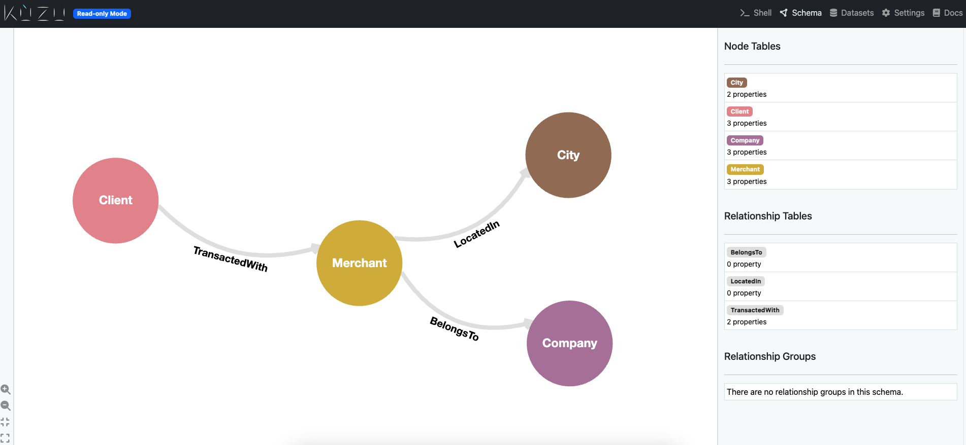
The above schema is very similar to the one we designed earlier, which is a good sign!
Visualize nodes and edges
The following query can be entered to visualize the graph.
MATCH (a)-[b]->(c)
RETURN * LIMIT 50;
The RETURN * keyword passes all the named variables in the query to the visualization engine which
then renders the graph as follows.

It’s possible to customize the visual style of the graph by clicking on the Settings tab on the top right.
Conclusions
The aim of this blog post is to show how to transform data that might exist in a typical relational system to a graph and load it into a Kuzu database. We also show how to visualize the graph and run some simple queries to test our data model.
What’s important to take away from this exercise is that using a graph database like Kuzu for the kinds of queries we ran above makes a lot of sense. The raw transaction data that may have been sitting in an RDBMS system wasn’t simple to reason about when it came to answering questions about connected entities. Doing so in SQL would have required multiple joins and subqueries, whereas the Cypher queries we wrote were more intuitive and easier to read. That being said, not all kinds of queries benefit from a graph data model, and there are many cases where SQL and RDBMS are right tools for the job.
Another key takeaway is that designing a graph data model is an iterative exercise. You may not get it right the first time, and that’s okay! The key is to have a good understanding of the data and the questions you want to answer, and to keep refining the model as you learn more about the data. Using an embeddable solution like Kuzu is really helpful in this regard, as you can quickly load the data and test your queries without having to worry about setting up servers or authentication.
In the next post, we’ll look at a larger dataset of a similar nature, to answer more complex questions about disputed transactions. In the meantime, give Kuzu a try out on your own data, and begin thinking about whether knowledge graphs are a good fit for your use case!
Code
The code to reproduce the workflow shown in this post can be found in the graphdb-demo repository. It uses Kuzu’s Python API, but you are welcome to use the client API of your choice.